Type 1 Error and Power Calculation for Association

Type 1 Error and Power Calculation for Association Analysis Pak Sham & Shaun Purcell Advanced Workshop Boulder, CO, 2005

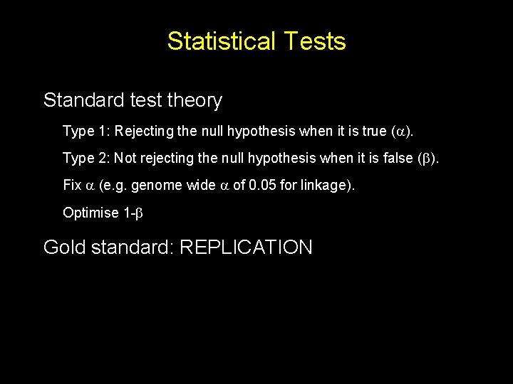
Statistical Tests Standard test theory Type 1: Rejecting the null hypothesis when it is true ( ). Type 2: Not rejecting the null hypothesis when it is false ( ). Fix (e. g. genome wide of 0. 05 for linkage). Optimise 1 - Gold standard: REPLICATION

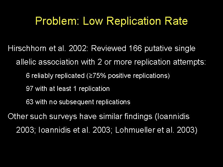
Problem: Low Replication Rate Hirschhorn et al. 2002: Reviewed 166 putative single allelic association with 2 or more replication attempts: 6 reliably replicated (≥ 75% positive replications) 97 with at least 1 replication 63 with no subsequent replications Other such surveys have similar findings (Ioannidis 2003; Ioannidis et al. 2003; Lohmueller et al. 2003)

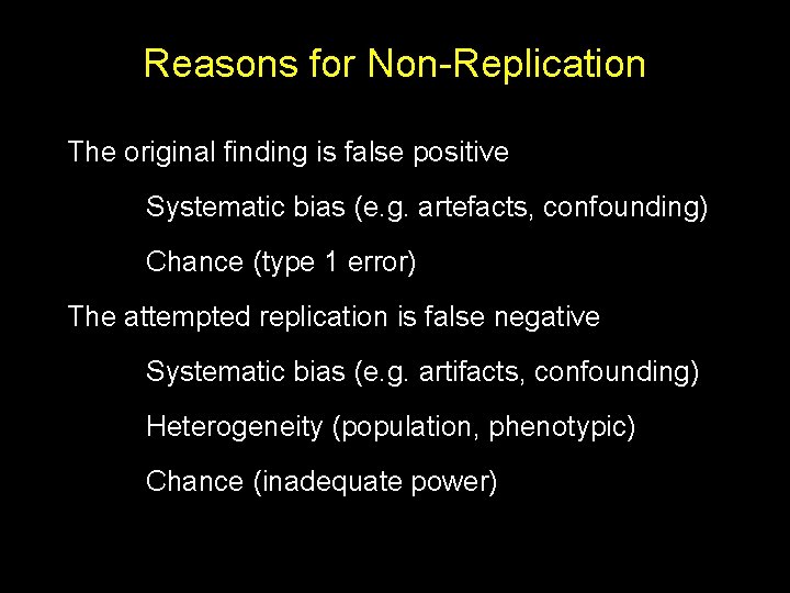
Reasons for Non-Replication The original finding is false positive Systematic bias (e. g. artefacts, confounding) Chance (type 1 error) The attempted replication is false negative Systematic bias (e. g. artifacts, confounding) Heterogeneity (population, phenotypic) Chance (inadequate power)

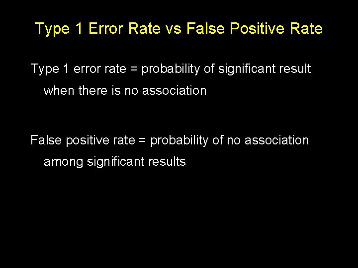
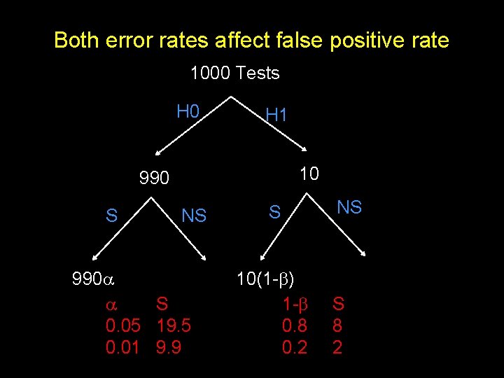
Type 1 Error Rate vs False Positive Rate Type 1 error rate = probability of significant result when there is no association False positive rate = probability of no association among significant results

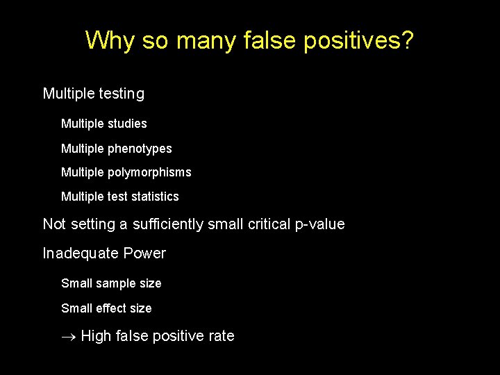
Why so many false positives? Multiple testing Multiple studies Multiple phenotypes Multiple polymorphisms Multiple test statistics Not setting a sufficiently small critical p-value Inadequate Power Small sample size Small effect size High false positive rate

Both error rates affect false positive rate 1000 Tests H 0 H 1 10 990 S NS 990 S 0. 05 19. 5 0. 01 9. 9 S 10(1 - ) 1 - 0. 8 0. 2 NS S 8 2

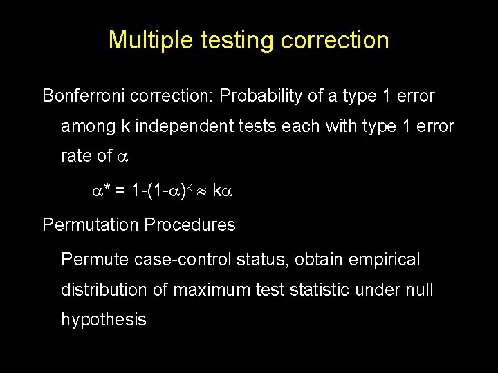
Multiple testing correction Bonferroni correction: Probability of a type 1 error among k independent tests each with type 1 error rate of * = 1 -(1 - )k k Permutation Procedures Permute case-control status, obtain empirical distribution of maximum test statistic under null hypothesis

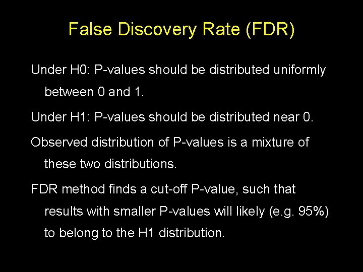
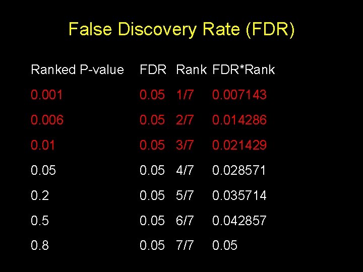
False Discovery Rate (FDR) Under H 0: P-values should be distributed uniformly between 0 and 1. Under H 1: P-values should be distributed near 0. Observed distribution of P-values is a mixture of these two distributions. FDR method finds a cut-off P-value, such that results with smaller P-values will likely (e. g. 95%) to belong to the H 1 distribution.

False Discovery Rate (FDR) Ranked P-value FDR Rank FDR*Rank 0. 001 0. 05 1/7 0. 007143 0. 006 0. 05 2/7 0. 014286 0. 01 0. 05 3/7 0. 021429 0. 05 4/7 0. 028571 0. 2 0. 05 5/7 0. 035714 0. 5 0. 05 6/7 0. 042857 0. 8 0. 05 7/7 0. 05

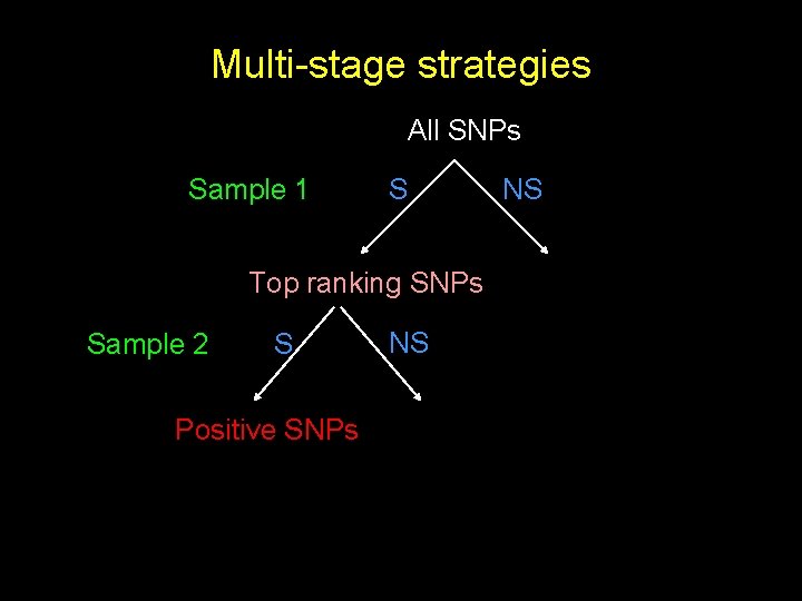
Multi-stage strategies All SNPs Sample 1 S Top ranking SNPs Sample 2 S Positive SNPs NS NS

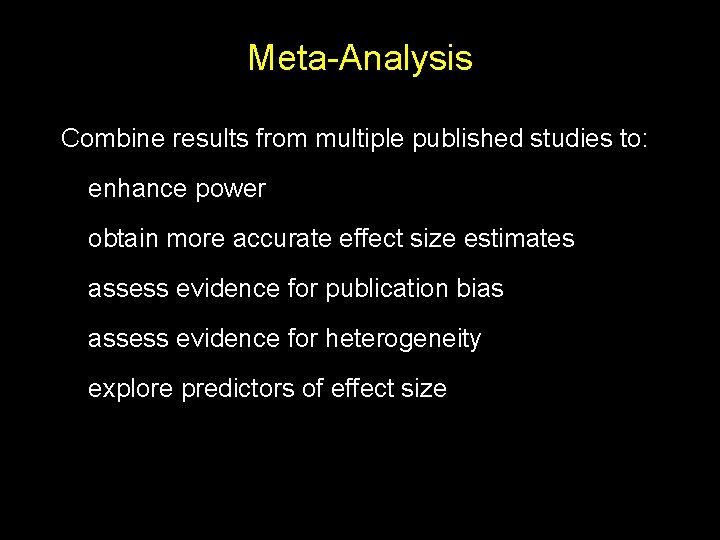
Meta-Analysis Combine results from multiple published studies to: enhance power obtain more accurate effect size estimates assess evidence for publication bias assess evidence for heterogeneity explore predictors of effect size

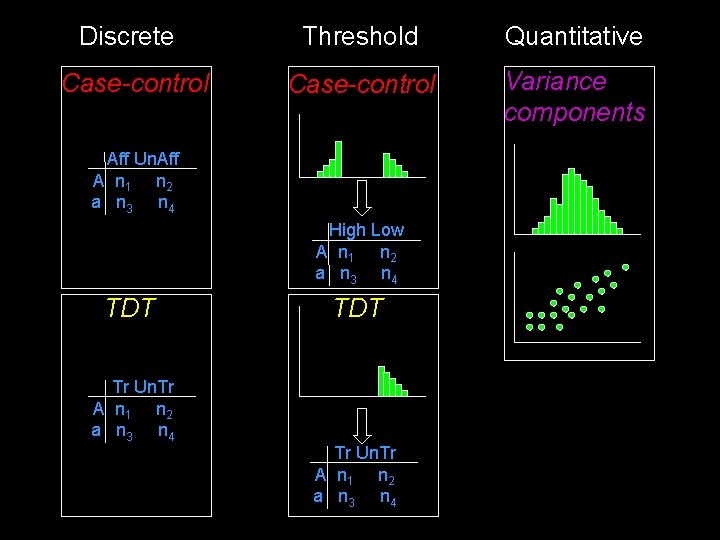
Discrete Case-control Threshold Quantitative Case-control Variance components Aff Un. Aff A n 1 n 2 a n 3 n 4 High Low A n 1 n 2 a n 3 n 4 TDT Tr Un. Tr A n 1 n 2 a n 3 n 4

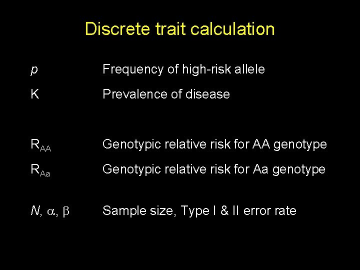
Discrete trait calculation p Frequency of high-risk allele K Prevalence of disease RAA Genotypic relative risk for AA genotype RAa Genotypic relative risk for Aa genotype N, , Sample size, Type I & II error rate

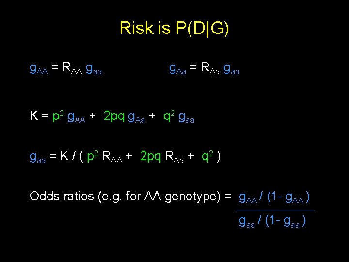
Risk is P(D|G) g. AA = RAA gaa g. Aa = RAa gaa K = p 2 g. AA + 2 pq g. Aa + q 2 gaa = K / ( p 2 RAA + 2 pq RAa + q 2 ) Odds ratios (e. g. for AA genotype) = g. AA / (1 - g. AA ) gaa / (1 - gaa )

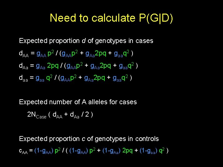
Need to calculate P(G|D) Expected proportion d of genotypes in cases d. AA = g. AA p 2 / (g. AAp 2 + g. Aa 2 pq + gaaq 2 ) d. Aa = g. Aa 2 pq / (g. AAp 2 + g. Aa 2 pq + gaaq 2 ) daa = gaa q 2 / (g. AAp 2 + g. Aa 2 pq + gaaq 2 ) Expected number of A alleles for cases 2 NCase ( d. AA + d. Aa / 2 ) Expected proportion c of genotypes in controls c. AA = (1 -g. AA) p 2 / ( (1 -g. AA) p 2 + (1 -g. Aa) 2 pq + (1 -gaa) q 2 )

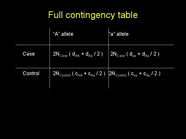
Full contingency table “A” allele “a” allele Case 2 NCase ( d. AA + d. Aa / 2 ) 2 NCase ( daa + d. Aa / 2 ) Control 2 NControl ( c. AA + c. Aa / 2 ) 2 NControl ( caa + c. Aa / 2 )

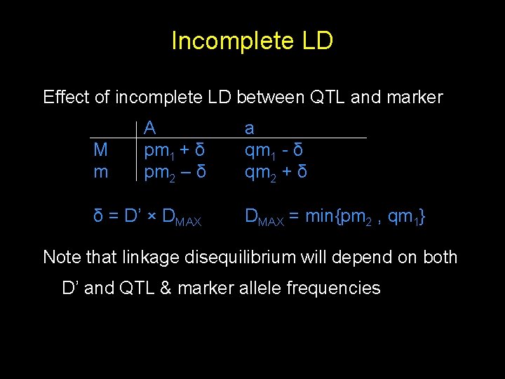
Incomplete LD Effect of incomplete LD between QTL and marker M m A pm 1 + δ pm 2 – δ δ = D’ × DMAX a qm 1 - δ qm 2 + δ DMAX = min{pm 2 , qm 1} Note that linkage disequilibrium will depend on both D’ and QTL & marker allele frequencies

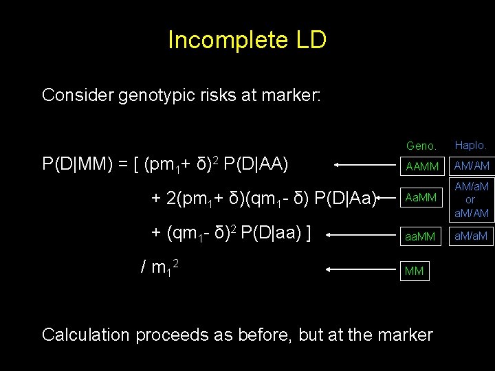
Incomplete LD Consider genotypic risks at marker: Geno. Haplo. AAMM AM/AM + 2(pm 1+ δ)(qm 1 - δ) P(D|Aa) Aa. MM AM/a. M or a. M/AM + (qm 1 - δ)2 P(D|aa) ] aa. MM a. M/a. M P(D|MM) = [ (pm 1+ δ)2 P(D|AA) / m 12 MM Calculation proceeds as before, but at the marker

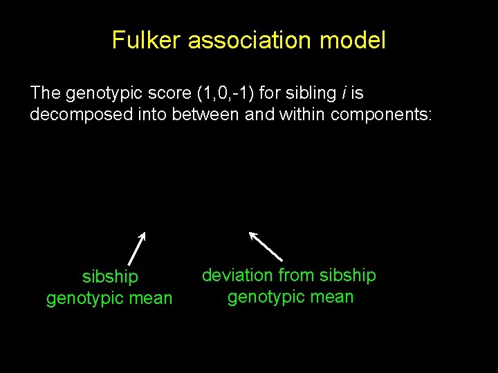
Fulker association model The genotypic score (1, 0, -1) for sibling i is decomposed into between and within components: sibship genotypic mean deviation from sibship genotypic mean

NCPs of B and W tests Approximation for between test Approximation for within test Sham et al (2000) AJHG 66

GPC Usual URL for GPC http: //statgen. iop. kcl. ac. uk/gpc/ Purcell S, Cherny SS, Sham PC. (2003) Genetic Power Calculator: design of linkage and association genetic mapping studies of complex traits. Bioinformatics, 19(1): 149 -50

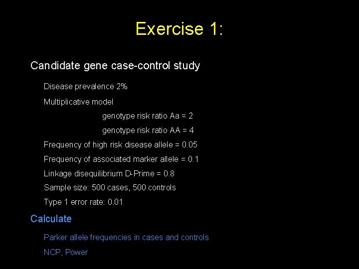
Exercise 1: Candidate gene case-control study Disease prevalence 2% Multiplicative model genotype risk ratio Aa = 2 genotype risk ratio AA = 4 Frequency of high risk disease allele = 0. 05 Frequency of associated marker allele = 0. 1 Linkage disequilibrium D-Prime = 0. 8 Sample size: 500 cases, 500 controls Type 1 error rate: 0. 01 Calculate Parker allele frequencies in cases and controls NCP, Power

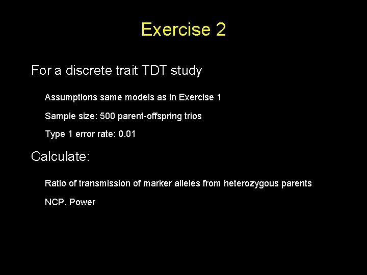
Exercise 2 For a discrete trait TDT study Assumptions same models as in Exercise 1 Sample size: 500 parent-offspring trios Type 1 error rate: 0. 01 Calculate: Ratio of transmission of marker alleles from heterozygous parents NCP, Power

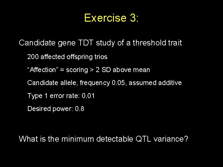
Exercise 3: Candidate gene TDT study of a threshold trait 200 affected offspring trios “Affection” = scoring > 2 SD above mean Candidate allele, frequency 0. 05, assumed additive Type 1 error rate: 0. 01 Desired power: 0. 8 What is the minimum detectable QTL variance?

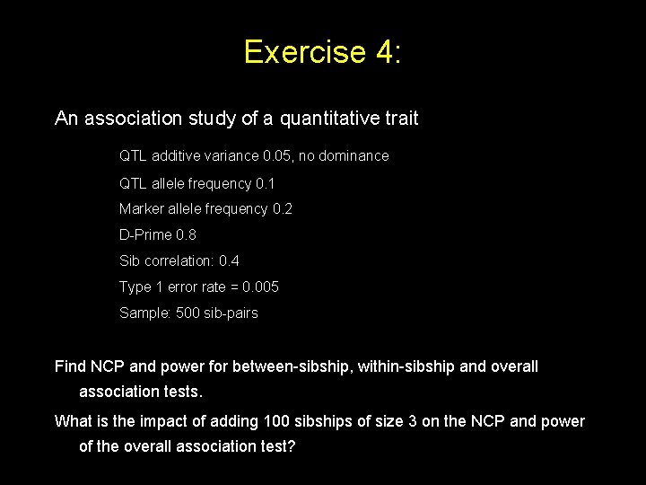
Exercise 4: An association study of a quantitative trait QTL additive variance 0. 05, no dominance QTL allele frequency 0. 1 Marker allele frequency 0. 2 D-Prime 0. 8 Sib correlation: 0. 4 Type 1 error rate = 0. 005 Sample: 500 sib-pairs Find NCP and power for between-sibship, within-sibship and overall association tests. What is the impact of adding 100 sibships of size 3 on the NCP and power of the overall association test?

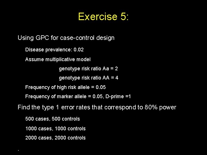
Exercise 5: Using GPC for case-control design Disease prevalence: 0. 02 Assume multiplicative model genotype risk ratio Aa = 2 genotype risk ratio AA = 4 Frequency of high risk allele = 0. 05 Frequency of marker allele = 0. 05, D-prime =1 Find the type 1 error rates that correspond to 80% power 500 cases, 500 controls 1000 cases, 1000 controls 2000 cases, 2000 controls .

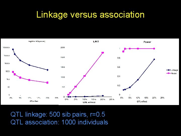
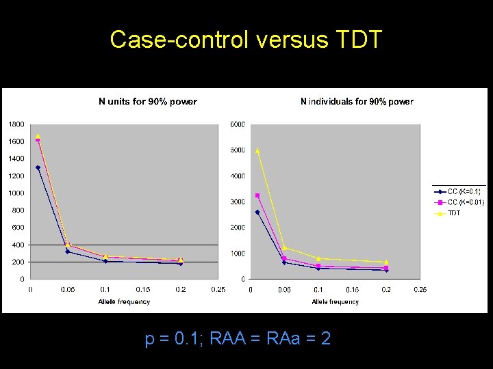
Exploring power of association using GPC Linkage versus association difference in required sample sizes for specific QTL size TDT versus case-control difference in efficiency? Quantitative versus binary traits loss of power from artificial dichotomisation?

Linkage versus association QTL linkage: 500 sib pairs, r=0. 5 QTL association: 1000 individuals

Case-control versus TDT p = 0. 1; RAA = RAa = 2

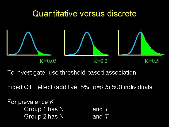
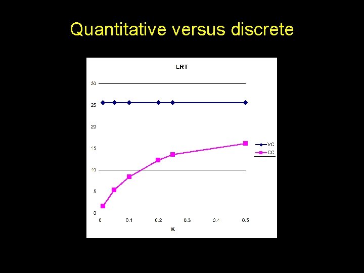
Quantitative versus discrete K=0. 05 K=0. 2 K=0. 5 To investigate: use threshold-based association Fixed QTL effect (additive, 5%, p=0. 5) 500 individuals For prevalence K Group 1 has N Group 2 has N and T

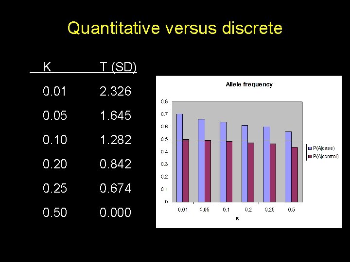
Quantitative versus discrete K T (SD) 0. 01 2. 326 0. 05 1. 645 0. 10 1. 282 0. 20 0. 842 0. 25 0. 674 0. 50 0. 000

Quantitative versus discrete

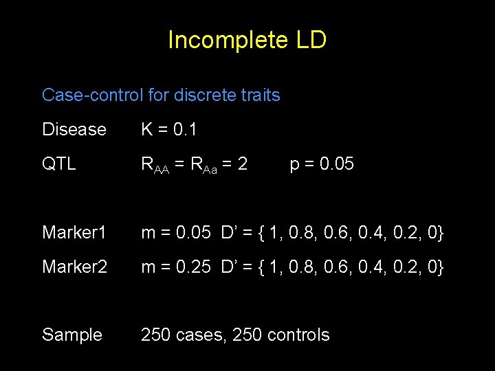
Incomplete LD what is the impact of D’ values less than 1? does allele frequency affect the power of the test? (using discrete case-control calculator) Family-based VC association: between and within tests what is the impact of sibship size? sibling correlation? (using QTL VC association calculator)

Incomplete LD Case-control for discrete traits Disease K = 0. 1 QTL RAA = RAa = 2 Marker 1 m = 0. 05 D’ = { 1, 0. 8, 0. 6, 0. 4, 0. 2, 0} Marker 2 m = 0. 25 D’ = { 1, 0. 8, 0. 6, 0. 4, 0. 2, 0} Sample 250 cases, 250 controls p = 0. 05

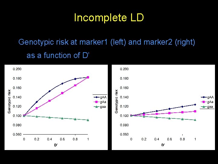
Incomplete LD Genotypic risk at marker 1 (left) and marker 2 (right) as a function of D’

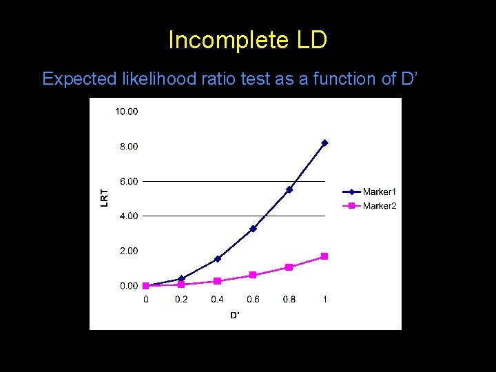
Incomplete LD Expected likelihood ratio test as a function of D’

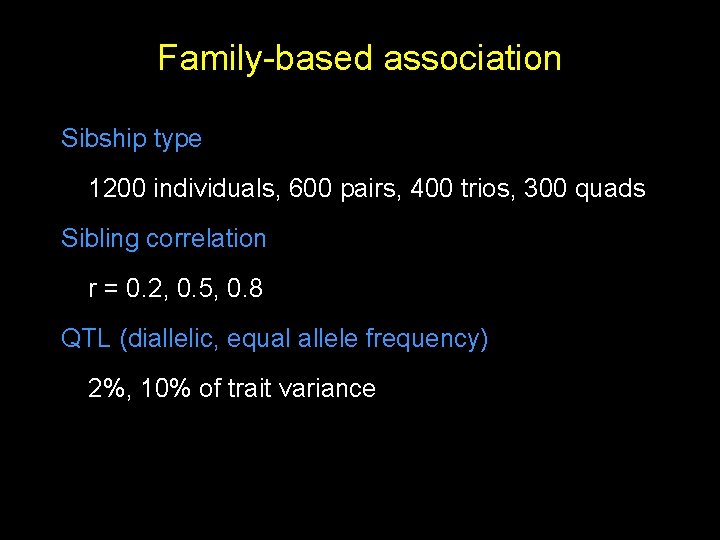
Family-based association Sibship type 1200 individuals, 600 pairs, 400 trios, 300 quads Sibling correlation r = 0. 2, 0. 5, 0. 8 QTL (diallelic, equal allele frequency) 2%, 10% of trait variance

Between-sibship association

Within-sibship association

Total association