TwoWay ANOVA Interactions What we will cover Twoway

Two-Way ANOVA Interactions

What we will cover • Two-way ANOVA: • • Family of ANOVA tests More examples in R Looking at interaction plots How to interpret the results

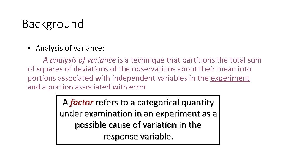
Background • Analysis of variance: A analysis of variance is a technique that partitions the total sum of squares of deviations of the observations about their mean into portions associated with independent variables in the experiment and a portion associated with error A factor refers to a categorical quantity under examination in an experiment as a possible cause of variation in the response variable.

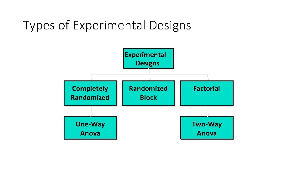
Types of Experimental Designs Completely Randomized One-Way Anova Randomized Block Factorial Two-Way Anova

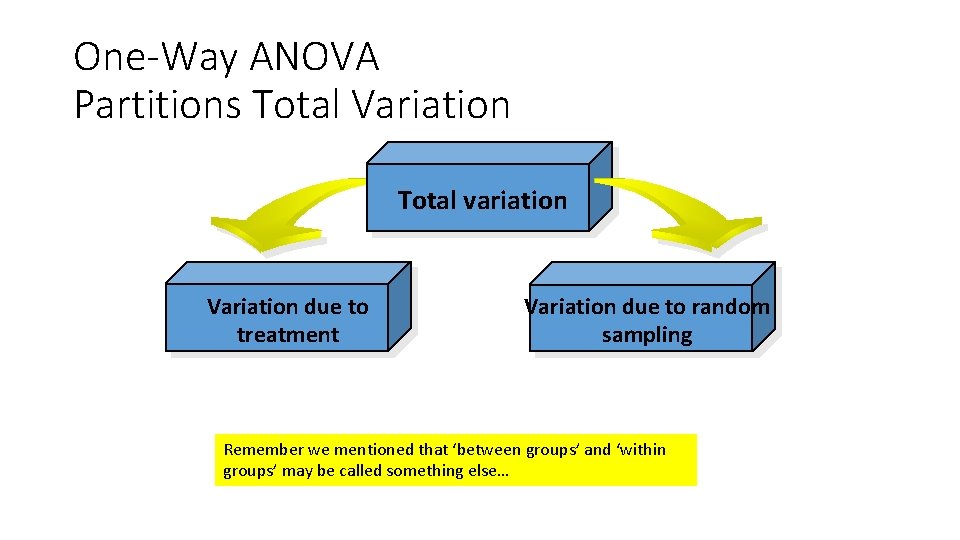
One-Way ANOVA Partitions Total Variation Total variation Variation due to treatment Variation due to random sampling Remember we mentioned that ‘between groups’ and ‘within groups’ may be called something else…

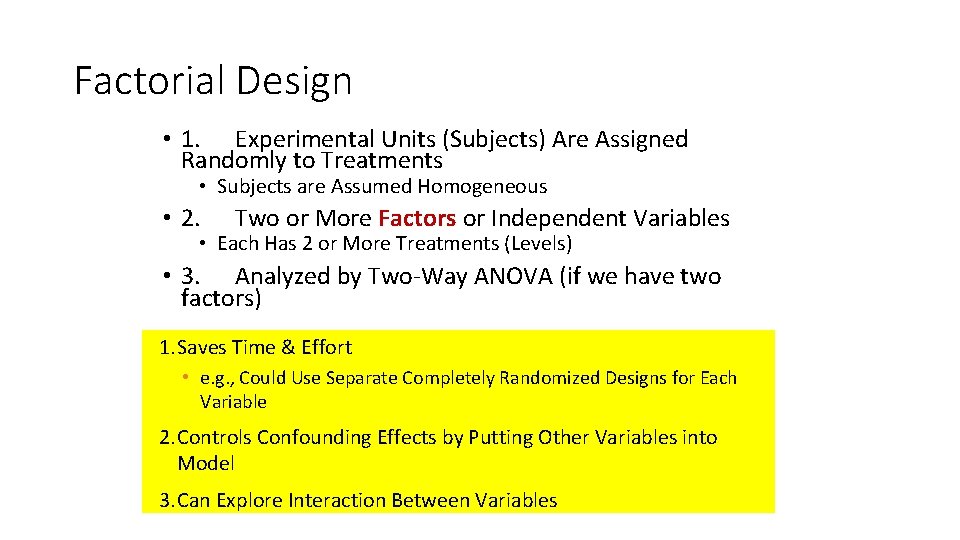
Factorial Design • 1. Experimental Units (Subjects) Are Assigned Randomly to Treatments • Subjects are Assumed Homogeneous • 2. Two or More Factors or Independent Variables • Each Has 2 or More Treatments (Levels) • 3. Analyzed by Two-Way ANOVA (if we have two factors) 1. Saves Time & Effort • e. g. , Could Use Separate Completely Randomized Designs for Each Variable 2. Controls Confounding Effects by Putting Other Variables into Model 3. Can Explore Interaction Between Variables

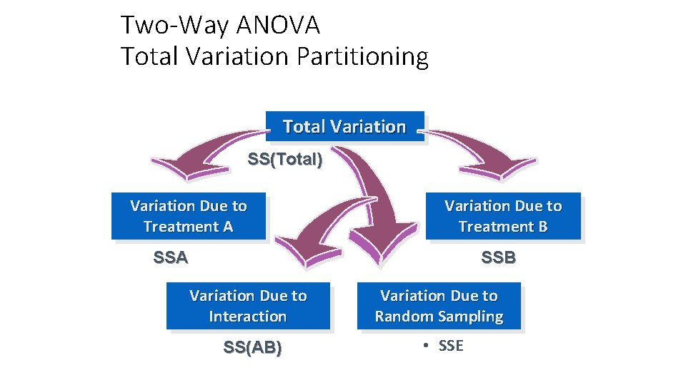
Two-Way ANOVA Total Variation Partitioning Total Variation SS(Total) Variation Due to Treatment A Variation Due to Treatment B SSA SSB Variation Due to Interaction Variation Due to Random Sampling SS(AB) • SSE

Part 2 – The two way ANOVA • Example Suppose you want to determine whether the brand of laundry detergent used and the temperature affects the amount of dirt removed from your laundry. • To this end, you buy two different brand of detergent (“ Super” and “Best”) and choose three different temperature levels (“cold”, “warm”, and “hot”). • Then you divide your laundry randomly into 6×r piles of equal size and assign each r piles into the combination of (“Super” and “Best”) and (”cold”, ”warm”, and “hot”).

Two-way ANOVA • A two-way ANOVA always involves two independent variables. • Each independent variable, or factor, is made up of, or defined by, two or more elements called levels. • When looked at simultaneously, the levels of the first factor and the levels of the second factor create the conditions of the study to be compared. • Each of these conditions is referred to as a cell.

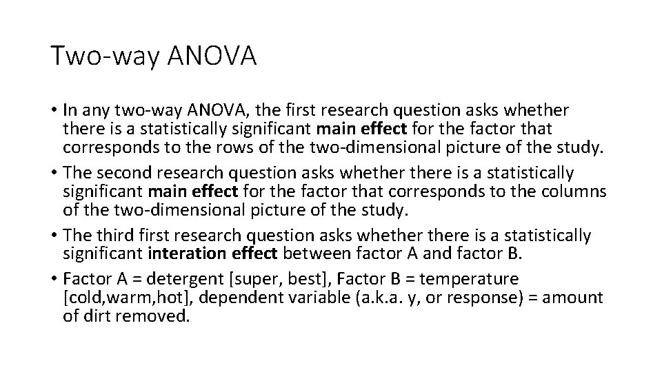
Two-way ANOVA • In any two-way ANOVA, the first research question asks whethere is a statistically significant main effect for the factor that corresponds to the rows of the two-dimensional picture of the study. • The second research question asks whethere is a statistically significant main effect for the factor that corresponds to the columns of the two-dimensional picture of the study. • The third first research question asks whethere is a statistically significant interation effect between factor A and factor B. • Factor A = detergent [super, best], Factor B = temperature [cold, warm, hot], dependent variable (a. k. a. y, or response) = amount of dirt removed.

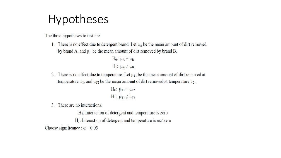
Hypotheses

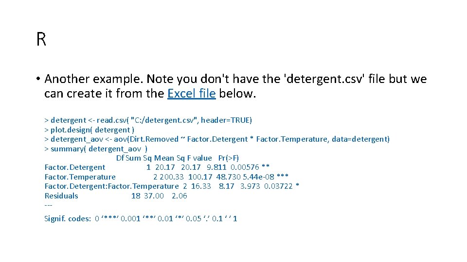
R • Another example. Note you don't have the 'detergent. csv' file but we can create it from the Excel file below. > detergent <- read. csv( "C: /detergent. csv", header=TRUE) > plot. design( detergent ) > detergent_aov <- aov(Dirt. Removed ~ Factor. Detergent * Factor. Temperature, data=detergent) > summary( detergent_aov ) Df Sum Sq Mean Sq F value Pr(>F) Factor. Detergent 1 20. 17 9. 811 0. 00576 ** Factor. Temperature 2 200. 33 100. 17 48. 730 5. 44 e-08 *** Factor. Detergent: Factor. Temperature 2 16. 33 8. 17 3. 973 0. 03722 * Residuals 18 37. 00 2. 06 --Signif. codes: 0 ‘***’ 0. 001 ‘**’ 0. 01 ‘*’ 0. 05 ‘. ’ 0. 1 ‘ ’ 1

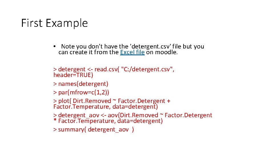
First Example • Note you don't have the 'detergent. csv' file but you can create it from the Excel file on moodle. > detergent <- read. csv( "C: /detergent. csv", header=TRUE) > names(detergent) > par(mfrow=c(1, 2)) > plot( Dirt. Removed ~ Factor. Detergent + Factor. Temperature, data=detergent) > detergent_aov <- aov(Dirt. Removed ~ Factor. Detergent * Factor. Temperature, data=detergent) > summary( detergent_aov )

Check the P-value • What is it? “The P value or calculated probability is the estimated probability of rejecting the null hypothesis (H 0) of a study question when that hypothesis is true. ” [http: //www. statsdirect. com/help/basics/pval. htm] “…p-value is the probability of finding the observed sample results, or "more extreme" results, when the null hypothesis is actually true (where "more extreme" is dependent on the way the hypothesis is tested)[http: //en. wikipedia. org/wiki/P-value] • Just think about what we are really doing! • We assume the null hypothesis is true

Reducing the Dataset • detergent_no_cold <- detergent[detergent$Factor. Temperature != 'cold', ] • detergent__no_cold_aov <- aov(Dirt. Removed ~ Factor. Detergent * Factor. Temperature, data=detergent_no_cold) • summary(detergent__no_cold_aov) • detergent_no_warm = subset(detergent, Factor. Temperature != 'warm') • View(detergent_no_cold) • View(detergent_no_warm) • detergent_no_temperature = detergent[c(1, 3)] • detergent_no_brand <- detergent[2: 3]

Calculations • The excel file shows where some of the values come from etc. • But this type of analysis is done with a stats package. • We can carry out the two-way ANOVA in excel too…

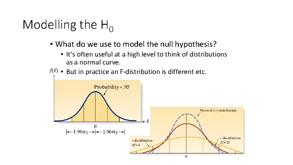
Modelling the H 0 • What do we use to model the null hypothesis? • It’s often useful at a high level to think of distributions as a normal curve. • But in practice an F-distribution is different etc.

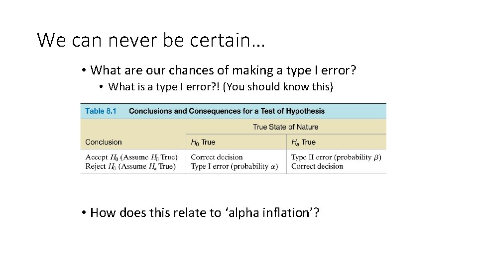
We can never be certain… • What are our chances of making a type I error? • What is a type I error? ! (You should know this) • How does this relate to ‘alpha inflation’?

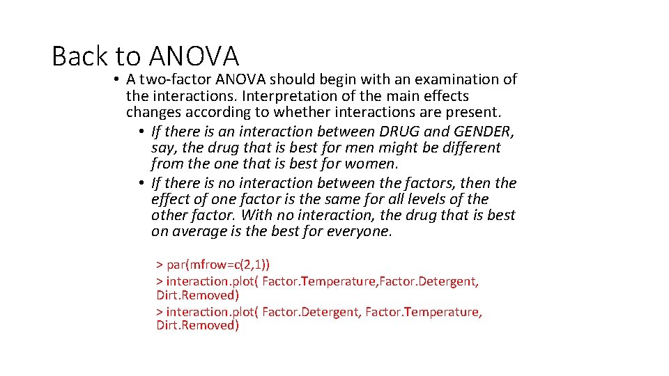
Back to ANOVA • A two-factor ANOVA should begin with an examination of the interactions. Interpretation of the main effects changes according to whether interactions are present. • If there is an interaction between DRUG and GENDER, say, the drug that is best for men might be different from the one that is best for women. • If there is no interaction between the factors, then the effect of one factor is the same for all levels of the other factor. With no interaction, the drug that is best on average is the best for everyone. > par(mfrow=c(2, 1)) > interaction. plot( Factor. Temperature, Factor. Detergent, Dirt. Removed) > interaction. plot( Factor. Detergent, Factor. Temperature, Dirt. Removed)

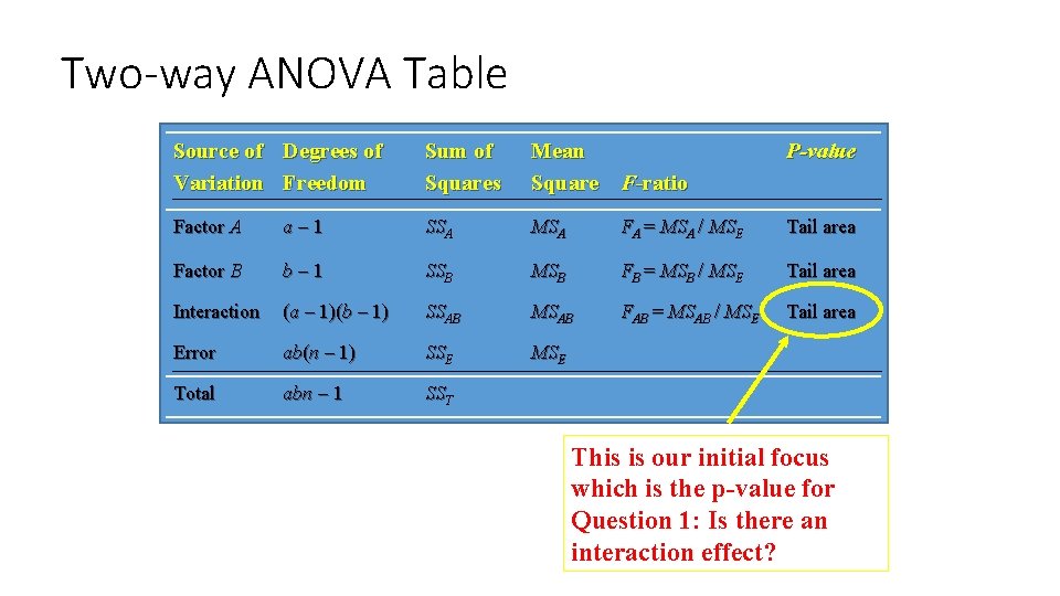
Two-way ANOVA Table Source of Degrees of Variation Freedom Sum of Squares Mean Square F-ratio P-value Factor A a-1 SSA MSA FA = MSA / MSE Tail area Factor B b-1 SSB MSB FB = MSB / MSE Tail area Interaction (a – 1)(b – 1) SSAB MSAB FAB = MSAB / MSE Tail area Error ab(n – 1) SSE MSE Total abn - 1 SST This is our initial focus which is the p-value for Question 1: Is there an interaction effect?

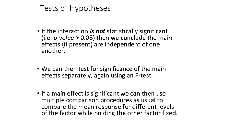
Tests of Hypotheses • If the interaction is not statistically significant (i. e. p-value > 0. 05) then we conclude the main effects (if present) are independent of one another. • We can then test for significance of the main effects separately, again using an F-test. • If a main effect is significant we can then use multiple comparison procedures as usual to compare the mean response for different levels of the factor while holding the other factor fixed.