TWOPERSON ZEROSUM GAMES Zerosum games one player wins

TWO-PERSON, ZERO-SUM GAMES Ø Zero-sum games : one player wins whatever the other one loses, so that the sum of their net winnings is zero. Ø The game: odds and evens. Ø This game consists simply of each player simultaneously showing either one finger or two fingers. Ø If the number of fingers matches, so that the total number for both players is even, then the player taking evens (say, player 1) wins the bet (say, $1) from the player taking odds (player 2). Ø If the number does not match, player 1 pays $1 to player 2. Ø each player has two strategies: to show either one finger or two fingers.

Two-person game Ø In general, a two-person game is characterized by: Ø The strategies of player 1 Ø The strategies of player 2 Ø The payoff table ØBefore the game begins, each player knows the strategies she or he has available, the ones the opponent has available, and the payoff table. Ø The actual play of the game consists of each player simultaneously choosing a strategy without knowing the opponent’s choice.

Strategy Ø In more complicated games involving a series of moves, a strategy is a predetermined rule that specifies completely how one intends to respond to each possible circumstance at each stage of the game. (e. g. Chess) Ø Applications of game theory normally involve far less complicated competitive situations than chess does, but the strategies involved can be fairly complex. Ø The payoff table shows the gain (positive or negative) for player 1 that would result from each combination of strategies for the two players.

Ø A primary objective of game theory is the development of rational criteria for selecting a strategy. Two key assumptions are made: Ø Both players are rational. Ø Both players choose their strategies solely to promote their own welfare (no compassion for the opponent).

PROTOTYPE EXAMPLE Ø To formulate this problem as a two-person, zero-sum game, we must identify the two players (obviously the two politicians), the strategies for each player, and the payoff table. Ø As the problem has been stated, each player has the following three strategies: Ø Strategy 1 spend 1 day in each city. Ø Strategy 2 spend both days in Bigtown. Ø Strategy 3 spend both days in Megalopolis.

Formulation as a Two-Person, Zero-Sum Game

Variation 1 ØThe answer can be obtained just by applying the concept of dominated strategies to rule out a succession of inferior strategies until only one choice remains. ØA strategy is dominated by a second strategy if the second strategy is always at least as good (and sometimes better) regardless of what the opponent does. ØA dominated strategy can be eliminated immediately from further consideration.

Variation 1 For player 1, strategy 3 is dominated by strategy 1 because the latter has larger payoffs (1 > 0, 2> 1, 4>1) regardless of what player 2 does. player 2 now does have a dominated strategy—strategy 3, which is dominated by both strategies 1 and 2, because they always have smaller losses for player 2 (payoffs to player 1) in this reduced payoff table (for strategy 1: 1 < 4, 1< 5; for strategy 2: 2< 4, 0< 5). At this point, strategy 2 for player 1 becomes dominated by strategy 1 because the latter is better in column 2 (2 > 0) and equally good in column 1 (1 =1). Strategy 2 for player 2 now is dominated by strategy 1 (1 <2), so strategy 2 should be eliminated

Variation 1 Ø Consequently, both players should select their strategy 1. Ø Player 1 then will receive a payoff of 1 from player 2 (that is, politician 1 will gain 1, 000 votes from politician 2). Ø In general, the payoff to player 1 when both players play optimally is referred to as the value of the game. Ø A game that has a value of 0 is said to be a fair game. Ø Since this particular game has a value of 1, it is not a fair game.

Variation 2 This game does not have dominated strategies

Ø Consider player 1. By selecting strategy 1, he could win 6 or could lose as much as 3. Ø However, because player 2 is rational and thus will seek a strategy that will protect himself from large payoffs to player 1, it seems likely that player 1 would incur a loss by playing strategy 1. Ø Similarly, by selecting strategy 3, player 1 could win 5, but more probably his rational opponent would avoid this loss and instead administer a loss to player 1 which could be as large as 4. Ø On the other hand, if player 1 selects strategy 2, he is guaranteed not to lose anything and he could even win something. Ø Therefore, because it provides the best guarantee (a payoff of 0), strategy 2 seems to be a “rational” choice for player 1 against his rational opponent. (This line of reasoning assumes that both players are averse to risking larger losses than necessary, in contrast to those individuals who enjoy gambling for a large payoff against long odds. )

Minimax criterion Ø The end product of this line of reasoning is that each player should play in such a way as to minimize his maximum losses whenever the resulting choice of strategy cannot be exploited by the opponent to then improve his position. Ø This so-called minimax criterion is a standard criterion proposed by game theory for selecting a strategy. Ø In terms of the payoff table, it implies that player 1 should select the strategy whose minimum payoff is largest, whereas player 2 should choose the one whose maximum payoff to player 1 is the smallest. Ø This criterion is illustrated in Table 14. 4, where strategy 2 is identified as the maximin strategy for player 1 and strategy 2 is the minimax strategy for player 2. Ø The resulting payoff of 0 is the value of the game, so this is a fair game.

saddle point Ø Notice the interesting fact that the same entry in this payoff table yields both the maximin and minimax values. Ø The reason is that this entry is both the minimum in its row and the maximum of its column. Ø The position of any such entry is called a saddle point. Ø Because of the saddle point, neither player can take advantage of the opponent’s strategy to improve his own position. Ø Since this is a stable solution (also called an equilibrium solution), players 1 and 2 should exclusively use their maximin and minimax strategies, respectively.

Variation 3 The result is that there is no saddle point. In short, the originally suggested solution (player 1 to play strategy 1 and player 2 to play strategy 3) is an unstable solution, so it is necessary to develop a more satisfactory solution

Variation 3 Ø Therefore, an essential feature of a rational plan for playing a game such as this one is that neither player should be able to deduce which strategy the other will use. Ø Hence, in this case, rather than applying some known criterion for determining a single strategy that will definitely be used, it is necessary to choose among alternative acceptable strategies on some kind of random basis. Ø By doing this, neither player knows in advance which of his own strategies will be used, let alone what his opponent will do. Ø This suggests, in very general terms, the kind of approach that is required for games lacking a saddle point.

Game with mixed strategies Ø Whenever a game does not possess a saddle point, game theory advises each player to assign a probability distribution over her set of strategies. Ø m and n are the respective numbers of available strategies Ø Player 1 would specify her plan for playing the game by assigning values to x 1, x 2, . . . , xm. Ø (x 1, x 2, . . . , xm) and (y 1, y 2, . . . , yn) are usually referred to as mixed strategies, and the original strategies are then called pure strategies.

Game with mixed strategies Ø Although no completely satisfactory measure of performance is available for evaluating mixed strategies, a very useful one is the expected payoff. By applying the probability theory definition of expected value Pij= the payoff if player 1 uses pure strategy i and player 2 uses pure strategy j. ØThus, this measure of performance does not disclose anything about the risks involved in playing the game, but it does indicate what the average payoff will tend to be if the game is played many times.

Game with mixed strategies Ø Extending the concept of the minimax criterion to games that lack a saddle point and thus need mixed strategies. Ø The minimax criterion says that a given player should select the mixed strategy that minimizes the maximum expected loss to himself. Ø Equivalently, when we focus on payoffs (player 1) rather than losses (player 2), this criterion says to maximin instead, i. e. , maximize the minimum expected payoff to the player.

Game with mixed strategies Ø By the minimum expected payoff we mean the smallest possible expected payoff that can result from any mixed strategy with which the opponent can counter. Ø Thus, the mixed strategy for player 1 that is optimal according to this criterion is the one that provides the guarantee (minimum expected payoff) that is best (maximal). (The value of this best guarantee is the maximin value, denoted by v. ) Ø Similarly, the optimal strategy for player 2 is the one that provides the best guarantee, where best now means minimal and guarantee refers to the maximum expected loss that can be administered by any of the opponent’s mixed strategies. (This best guarantee is the minimax value, denoted by v. )

Game with mixed strategies Ø Recall that when only pure strategies were used, games not having a saddle point turned out to be unstable (no stable solutions). Ø The reason was essentially that Vmin<Vmax, so that the players would want to change their strategies to improve their positions. Similarly, for games with mixed strategies, it is necessary that v v for the optimal solution to be stable. Ø Fortunately, according to the minimax theorem of game theory, this condition always holds for such games

Minimax theorem Ø If mixed strategies are allowed, the pair of mixed strategies that is optimal according to the minimax criterion provides a stable solution with Vmin=Vmax=V , so that neither player can do better by unilaterally changing her or his strategy. Ø The only way to guarantee attaining the optimal expected payoff V is to randomly select the pure strategy to be used from the probability distribution for the optimal mixed strateg Ø How to find the optimal mixed strategy for each player. Ø There are several methods of doing this. (A graphical procedure that may be used whenever one of the players has only two (undominated) pure strategies; Ø When larger games are involved, the usual method is to transform the problem to a linear programming problem.

GRAPHICAL SOLUTION PROCEDURE mixed strategies are (x 1, x 2) and x 2 =1 - x 1, it is necessary to solve only for the optimal value of x 1 However, it is straightforward to plot the expected payoff as a function of x 1 for each of her opponent’s pure strategies. This graph can then be used to identify the point that maximizes the minimum expected payoff.

GRAPHICAL SOLUTION For each of the pure strategies available to player 2, the expected payoff for player 1 will be: Expected payoff for player 1= y 1(5 - 5 x 1)+ y 2(4 - 6 x 1) + y 3(3 - 5 x 1).

GRAPHICAL SOLUTION Ø Given x 1, player 2 can minimize this expected payoff by choosing the pure strategy that corresponds to the “bottom” line for that x 1 in Fig. 14. 1 (either -3 + 5 x 1 or 4 - 6 x 1, but never 5 -5 x 1). Ø According to the minimax (or maximin) criterion, player 1 wants to maximize this minimum expected payoff. Consequently, player 1 should select the value of x 1 where the bottom line peaks, i. e. , where the (-3+ 5 x 1) and (4 - 6 x 1) lines intersect, which yields an expected payoff of To solve algebraically for this optimal value of x 1 at the intersection of the two lines -3 + 5 x 1 and 4 - 6 x 1, we set -3+ 5 x 1= 4 - 6 x 1 is the value of the game

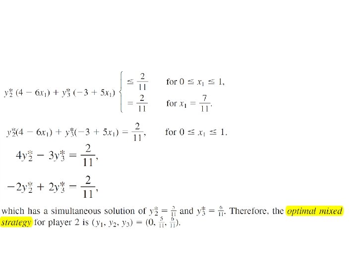
GRAPHICAL SOLUTION Ø According to the definition of the minimax value Vmax and the minimax theorem, the expected payoff resulting from the optimal strategy (y 1, y 2, y 3) = (y*1, y*2, y*3) will satisfy the condition Furthermore, when player 1 is playing optimally (that is, x 1=7/11), this inequality will be an equality (by the minimax theorem), so that Because (y 1, y 2, y 3) is a probability distribution, it is also known that Therefore, y*1= 0 because y*1> 0 would violate the next-to-last equation

SOLVING BY LINEAR PROGRAMMING Ø Any game with mixed strategies can be solved by transforming the problem to a linear programming problem. Ø This transformation requires little more than applying the minimax theorem and using the definitions of the maximin value v and minimax value Vmax. for all opposing strategies (y 1, y 2, . . . , yn). Thus, this inequality will need to hold, e. g. , for each of the pure strategies of player 2, that is, for each of the strategies (y 1, y 2, . . . , yn) where one yj= 1 and the rest equal 0. Substituting these values into the inequality yields:

SOLVING BY LINEAR PROGRAMMING Ø so that the inequality implies this set of n inequalities. Ø Furthermore, this set of n inequalities implies the original inequality (rewritten): Consequently, the problem of finding an optimal mixed strategy has been reduced to finding a feasible solution for a linear programming problem. The two remaining difficulties are that (1) v is unknown and (2) the linear programming problem has no objective function. Fortunately, both these difficulties can be resolved at one stroke by replacing the unknown constant v by the variable xm 1 and then maximizing xm 1, so that xm 1 automatically will equal v (by definition) at the optimal solution for the linear programming problem.

SOLVING BY LINEAR PROGRAMMING Ø To summarize, player 1 would find his optimal mixed strategy by using the simplex method to solve the linear programming problem:

SOLVING BY LINEAR PROGRAMMING optimal mixed strategy for player 2

Example

Example

Example Ø When the simplex method was applied to both of these linear programming models, a nonnegativity constraint was added that assumed that v 0. Ø If this assumption were violated, both models would have no feasible solutions, so the simplex method would stop quickly with this message. Ø To avoid this risk, we could have added a positive constant, say, 3 (the absolute value of the largest negative entry), to all the entries in Table 14. 6. Ø This then would increase by 3 all the coefficients of x 1, x 2, y 1, y 2, and y 3 in the inequality constraints of the two models

Extensions Ø Although this chapter has considered only two-person, zero -sum games with a finite number of pure strategies, game theory extends far beyond this kind of game. Ø In fact, extensive research has been done on a number of more complicated types of games, including the ones summarized in this section. Ø The simplest generalization is to the two-person, constantsum game. In this case, the sum of the payoffs to the two players is a fixed constant (positive or negative) regardless of which combination of strategies is selected. Ø The only difference from a two-person, zero-sum game is that, in the latter case, the constant must be zero.

Extensions Ø A nonzero constant may arise instead because, in addition to one player winning whatever the other one loses, the two players may share some reward (if the constant is positive) or some cost (if the constant is negative) for participating in the game. Ø Adding this fixed constant does nothing to affect which strategies should be chosen. Ø Therefore, the analysis for determining optimal strategies is exactly the same as described in this chapter for two-person, zerosum games.

n-person game Ø A more complicated extension is to the n-person game, where more than two players may participate in the game. Ø This generalization is particularly important because, in many kinds of competitive situations, frequently more than two competitors are involved. Ø This may occur, e. g. , in competition among business firms, in international diplomacy, and so forth. Ø Unfortunately, the existing theory for such games is less satisfactory than it is for two-person games.

nonzero-sum game Ø Another generalization is the nonzero-sum game, where the sum of the payoffs to the players need not be 0 (or any other fixed constant). Ø This case reflects the fact that many competitive situations include noncompetitive aspects that contribute to the mutual advantage or mutual disadvantage of the players. Ø For example, the advertising strategies of competing companies can affect not only how they will split the market but also the total size of the market for their competing products. Ø However, in contrast to a constant sum game, the size of the mutual gain (or loss) for the players depends on the combination of strategies chosen.

nonzero-sum game Ø Because mutual gain is possible, nonzero-sum games are further classified in terms of the degree to which the players are permitted to cooperate. Ø At one extreme is the noncooperative game, where there is no preplay communication between the players. Ø At the other extreme is the cooperative game, where preplay discussions and binding agreements are permitted. Ø For example, competitive situations involving trade regulations between countries, or collective bargaining between labor and management, might be formulated as cooperative games. Ø When there are more than two players, cooperative games also allow some of or all the players to form coalitions.

infinite games Ø Still another extension is to the class of infinite games, where the players have an infinite number of pure strategies available to them. Ø These games are designed for the kind of situation where the strategy to be selected can be represented by a continuous decision variable. Ø For example, this decision variable might be the time at which to take a certain action, or the proportion of one’s resources to allocate to a certain activity, in a competitive situation.