TwoGroup Discriminant Function Analysis Overview You wish to

Two-Group Discriminant Function Analysis

Overview • • You wish to predict group membership. There are only two groups. Your predictor variables are continuous. You will create a discriminant function, D, such that the two groups differ as much as possible on D.

The Discriminant Function • Weights are chosen such that were you to compute D for each case and then use ANOVA to compare the groups on D, the ratio of SSbetween to SSwithin would be as large as possible. • The value of this ratio is the eigenvalue.

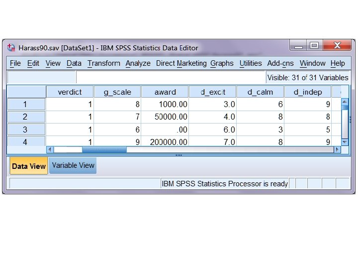
Harass 90. sav • Data are from Castellow, W. A. , Wuensch, K. L. , & Moore, C. H. (1990). Effects of physical attractiveness of the plaintiff and defendant in sexual harassment judgments. Journal of Social Behavior and Personality, 5, 547‑ 562. • Download from my SPSS Data page. • Bring into SPSS. Look at the data sheet.

The Variables • Verdict is mock juror’s recommendation, guilty (finding in favor of the plaintiff) or not (favor of defendant) • d_excit through d_happy are ratings of the defendant on various characteristics. • p_excit through p_happy are ratings of the plaintiff on the same characteristics.

Do the Analysis • Click Analyze, Classify, Discriminant. • Put all 22 rating scales (d_excit through p_happy) in the “Independents” box. • Put verdict into the “Grouping variable” box.

Now click on “verdict(? ? )” and then on “Define Range. ”

Enter “ 1” (Guilty) and “ 2” (Not) Click Continue. Back on the initial page, click “Statistics. ”

Check all of the Descriptives and Function Coefficients. Click Continue. Back on the initial page, click “Classify. ”

Select “Compute from group sizes” for the Priors and “Summary Table” for Display. Click Continue. Back on the initial page, click “Save. ”

Check “Discriminant scores” then click “Continue. ” Back on the initial page, click “OK. ”

Group Means • The Statistical Output • Look at the Group Statistics. – Mean ratings of defendant are more favorable in the Not Guilty group than in the Guilty group. – Mean ratings of the plaintiff are more favorable in the Guilty group than in the Not Guilty group.

Univariate ANOVAs • Look at the “Tests of Equality of Group Means. ” – The groups differ significantly on all but four of the variables.

Box’s M • Look at “Box’s Test of Equality of Covariance Matrices. ” • The null is that the variance-covariance matrix for the predictors is, in the populations, the same in both groups. • This is assumed when pooling these matrices during the DFA. • Box’s M is very powerful.

• We generally do not worry unless M is significant at. 001. Our p is. 002. • We may use elect to use Pillai’s Trace as the test statistic, as it is more robust to violation of this assumption. • Classification may be more affected by violation of this assumption than are the tests of significance.

ANOVA on the Discriminant Scores • Compare the two groups on the discriminant scores. Obtain • SSbetween groups • SSwithin groups • SStotal

Eigenvalue and Canonical Correlation • Look at the “Eigenvalues. ” – The eigenvalue, 1. 187, is for comparing the groups on the discriminant function. – The canonical correlation, . 737, is and is equivalent to eta from the ANOVA on D or point-biserial r beteen Groups and D.

Wilks’ Lambda • This is • 1 = eta-squared = 1 . 457 =. 543 • Eta-squared = canonical corr squared =. 7372 =. 543 • The grouping variable accounts for 54% of the variance in D.

Test of Significance • The smaller , the more doubt cast on the null that the groups do not differ on D. • Chi-square is used to test that null. It is significant. F can also be used. • There are other multivariate tests (such as Pillai’s trace) available elsewhere.

ANOVA on D • Click Analyze, Compare Means, One-Way ANOVA. • Put Verdict in the “Factor Box, ” the Discriminant scores in the “Dependent” list. Click OK.

• SSBetween SSWithin = 169. 753 143 = 1. 187 = the eigenvalue. • SSBetween SSTotal = 169. 753 312. 753 =. 543 = eta-squared = SQRT(Can. Corr) = SQRT(. 737) =. 543 = 1 . 457 =. 543.

Correlate D With Groups • Analyze, Correlate, Bivariate. • Click OK. r =. 737 = Canonical Correlation

Canonical Discriminant Function Coefficients • SPSS gives us both the standardized weights • And the unstandardized weights

DFC Weights vs Loadings • The usual cautions apply to the weights – for example, redundancy among predictors will reduce the values of weights. • The loadings in the structure matrix provide a better picture of how the discriminant function relates to the original variables.

The Loadings • These are correlations between D and the predictor variables. • For our data, high D is associated with the defendant being rated as socially desirable and the plaintiff being rated as socially undesirable.

The Loadings • The predictors with the highest positive loadings are D_sincerity (. 572), D_kindness (. 494), D_happiness (. 434), and D_warmth (. 420). • The predictors with the lowest negative loadings are P_warmth (-. 561), P_sincerity (-. 496), and P_kindness (-. 459).

High Scores on D Indicate • The respondent thinks the defendant is sincere, kind, happy, and warm. • And the plaintiff is cold, insincere, and mean

Group Centroids • These are simply the group means on D. • For those who found in favor of the defendant, D was high: + 1. 491. • For those who found in favor of the plaintiff, D was low: . 785.

Bayes Rule • For each case, probability of membership for each group is computed from the priors – p(Gi) – and the likelihoods – p(D|Gi).

Classification • Each case is classified into the group for which the posterior probability – p(Gi|D) – is greater. • By default, SPSS uses equal priors – for two groups, that would be. 5. • We asked that priors be computed from group frequencies, which should result in better classification.

Prior Probabilities • Cruising down Greenville Blvd. • What is the probability that the driver of the car ahead of you is male? • Assuming no sex differences in driving on the Blvd, prior prob =. 5

More information, this is the car:

Posterior Probabilities • Given that new information, what is the probability that the driver is male?

Prior Probabilities • Look at “Prior Probabilities for Groups. ” • As you can see, 65. 5% of the subjects voted Guilty, 34. 5% Not Guilty. • Using this information should produce better classification.

(Fisher’s) Classification Function Coefficients • For each case, two scores are computed from the weights and the subject’s scores on the variables. • D 1 is the score for Group 1 • D 2 is the score for Group 2 • If D 1 > D 2, the case is classified into Group 1. • If D 2 > D 1, into Group 2.

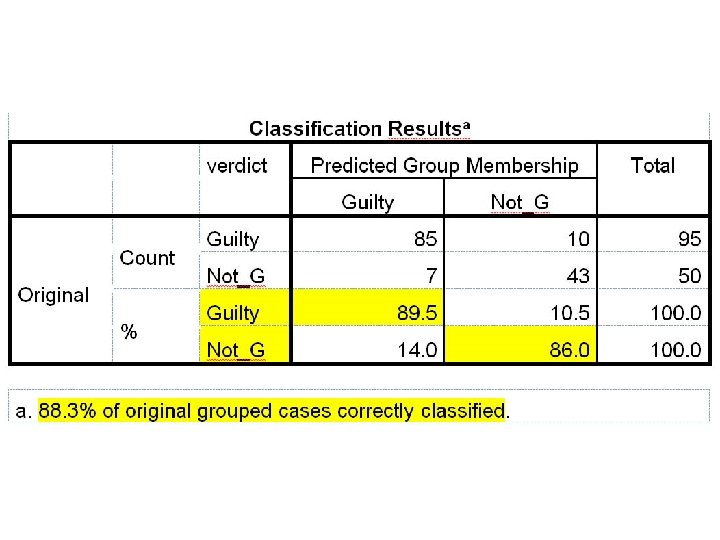
Classification Results • This table shows how well the classification went. • Of the 95 subjects who voted Guilty, 85 were correctly classified – 89. 5% success. • Of the 50 subjects who voted Not Guilty, 43 were correctly classified – 86%. • Overall, 88. 3% were correctly classified.

How Well Would We Have Done Just By Guessing? • Random Guessing – for each case, flip a fair coin. Heads you predict Group 1, tails Group 2. • P(Correct) =. 5(. 655) +. 5(. 345) = 50%

Probability Matching • In a situation like this, human guessers tend to take base rates into account, guessing for one or the other option in proportion to how frequently those guesses are correct. • P(Correct) =. 655(. 655) +. 345(. 345) = 55% correct.

Probability Maximizing • In this situation goldfish guess the more frequent option every time, and outperform humans. • P(Correct) = 65. 5%

Assumptions • Multivariate normality • Equality of variance-covariance matrices across groups

SAS • Download Harass 90. dat and DFA 2. sas. • Edit the program to point to the data file and run the program. • The output is essentially the same as that from SPSS, but arranged differently. • “Likelihood Ratio” is Wilks Lambda.

• For loadings and coefficients, use the “Pooled Within” tables. • Classification Results for Calibration Data – here are the posterior probabilities for misclassifications.

Multiple Regression to Predict Verdict • Look at the Proc Reg statement. • This is a simple multiple regression to predict verdict from the ratings variables. • The R-square = eta-squared from the DFA • SSmodel SSerror = the eigenvalue from the DFA. • SSerror SStotal = .

• The parameter estimates (unstandardized slopes) are perfectly correlated with the DFA coefficients. • Multiply any of the multiple regression parameter estimates by 4. 19395 and you get the DFA unstandardized coefficient.

MANOVA • Structurally identical to a DFA • DFA: Predict group membership from a set of continuous predictors. • MANOVA: Predict continuous predictors from group membership.

Logit Analysis • Predict group membership from two more categorical predictors. • Is basically a multivariate contingency table analysis, • But the effects included in the model are only those that involve the predicted (“dependent”) variable.

Logistic Regression • Predict group membership from two or more predictors. • Predictors can be categorical, continuous, or a mixture of categorical and continuous. • The assumptions are less restrictive than with DFA.