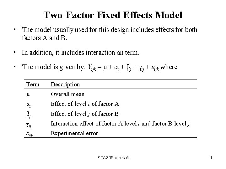
TwoFactor Fixed Effects Model The model usually used

Two-Factor Fixed Effects Model • The model usually used for this design includes effects for both factors A and B. • In addition, it includes interaction an term. • The model is given by: Yijk = μ + αi + βj + γij + εijk where Term Description μ Overall mean αi Effect of level i of factor A βj Effect of level j of factor B γij Interaction effect of factor A level i and factor B level j εijk Experimental error STA 305 week 5 1

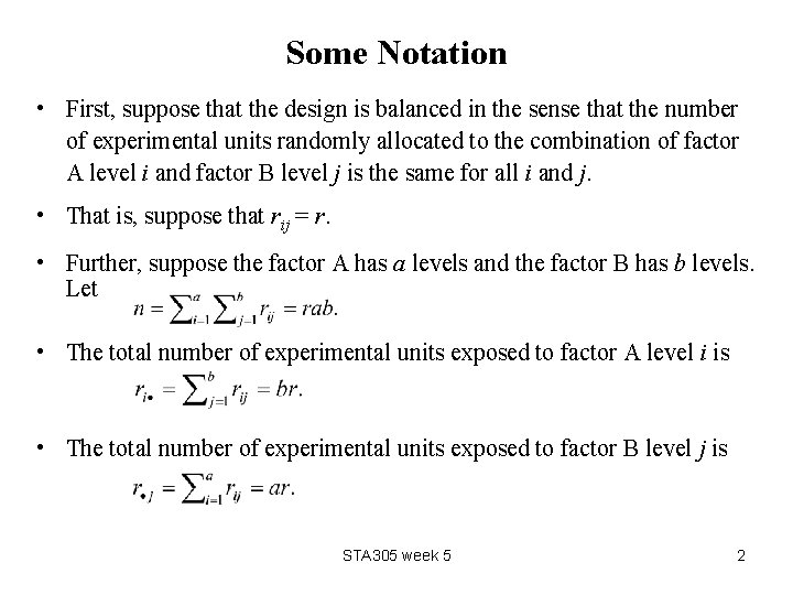
Some Notation • First, suppose that the design is balanced in the sense that the number of experimental units randomly allocated to the combination of factor A level i and factor B level j is the same for all i and j. • That is, suppose that rij = r. • Further, suppose the factor A has a levels and the factor B has b levels. Let • The total number of experimental units exposed to factor A level i is • The total number of experimental units exposed to factor B level j is STA 305 week 5 2

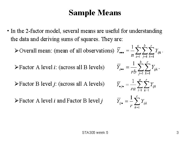
Sample Means • In the 2 -factor model, several means are useful for understanding the data and deriving sums of squares. They are: ØOverall mean: (mean of all observations) ØFactor A level i: (across all B levels) ØFactor B level j: (across all A levels) ØFactor A level i and Factor B level j STA 305 week 5 3

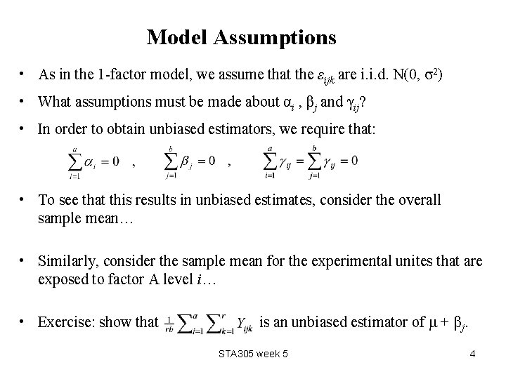
Model Assumptions • As in the 1 -factor model, we assume that the εijk are i. i. d. N(0, σ2) • What assumptions must be made about αi , βj and γij? • In order to obtain unbiased estimators, we require that: • To see that this results in unbiased estimates, consider the overall sample mean… • Similarly, consider the sample mean for the experimental unites that are exposed to factor A level i… • Exercise: show that is an unbiased estimator of μ + βj. STA 305 week 5 4

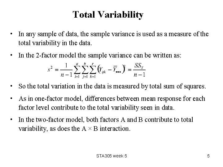
Total Variability • In any sample of data, the sample variance is used as a measure of the total variability in the data. • In the 2 -factor model the sample variance can be written as: • So the total variation in the data is measured by total sum of squares. • As in one-factor model, differences between mean response for each factor level contribute to the total variability seen in data. • In the two-factor model, both factors A and B contribute to total variability, as does the A × B interaction. STA 305 week 5 5

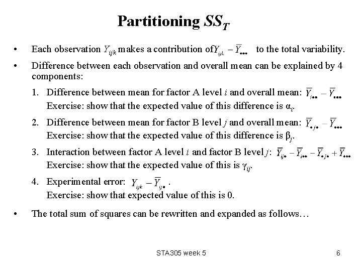
Partitioning SST • Each observation Yijk makes a contribution of • Difference between each observation and overall mean can be explained by 4 components: to the total variability. 1. Difference between mean for factor A level i and overall mean: Exercise: show that the expected value of this difference is αi. 2. Difference between mean for factor B level j and overall mean: Exercise: show that the expected value of this difference is βj. 3. Interaction between factor A level i and factor B level j: Exercise: show that the expected value of this is γij. 4. Experimental error: . Exercise: show that expected value of this is 0. • The total sum of squares can be rewritten and expanded as follows… STA 305 week 5 6

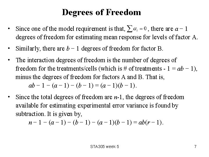
Degrees of Freedom • Since one of the model requirement is that, , there a − 1 degrees of freedom for estimating mean response for levels of factor A. • Similarly, there are b − 1 degrees of freedom for factor B. • The interaction degrees of freedom is the number of degrees of freedom for the treatments/cells (which is # of treatments - 1 = ab − 1), minus the degrees of freedom for factors A and B. That is, ab − 1 − (a − 1) − (b − 1) = (a − 1)(b − 1). • Since the total degrees of freedom are n-1, the degrees of freedom available for estimating experimental error variance is found by subtraction. It is given by, n − 1 − (a − 1) − (b − 1) − (a − 1)(b − 1) = ab(r − 1). STA 305 week 5 7

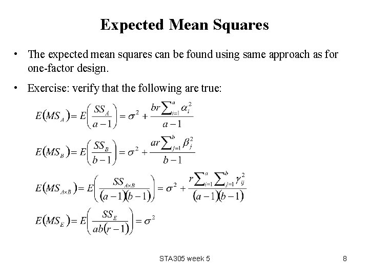
Expected Mean Squares • The expected mean squares can be found using same approach as for one-factor design. • Exercise: verify that the following are true: STA 305 week 5 8

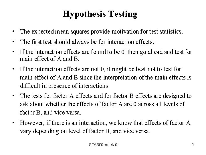
Hypothesis Testing • The expected mean squares provide motivation for test statistics. • The first test should always be for interaction effects. • If the interaction effects are found to be 0, then go ahead and test for main effect of A and B. • If the interaction effects are not 0, it might be best not to test for main effect of A and B since the interpretation of the main effects is difficult in presence of interactions. • The tests for factor A effects and for factor B effects are designed to ask about whether the effects of factor A are 0 across all levels of factor B, and vice versa. • However, if there is an interaction, we know that effects of factor A vary depending on level of factor B, and vice versa. STA 305 week 5 9

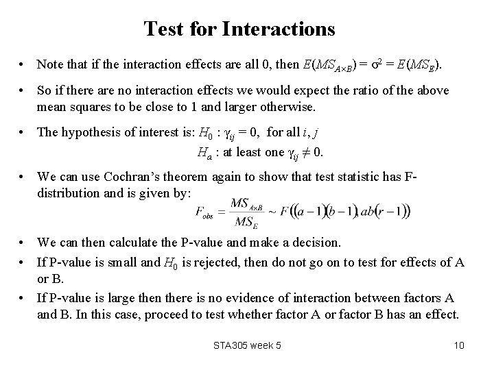
Test for Interactions • Note that if the interaction effects are all 0, then E(MSA×B) = σ2 = E(MSE). • So if there are no interaction effects we would expect the ratio of the above mean squares to be close to 1 and larger otherwise. • The hypothesis of interest is: H 0 : γij = 0, for all i, j Ha : at least one γij ≠ 0. • We can use Cochran’s theorem again to show that test statistic has Fdistribution and is given by: • We can then calculate the P-value and make a decision. • If P-value is small and H 0 is rejected, then do not go on to test for effects of A or B. • If P-value is large then there is no evidence of interaction between factors A and B. In this case, proceed to test whether factor A or factor B has an effect. STA 305 week 5 10

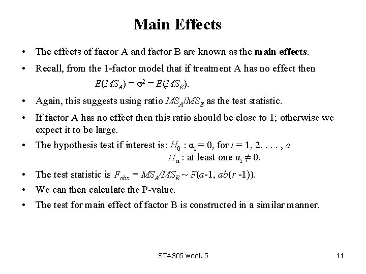
Main Effects • The effects of factor A and factor B are known as the main effects. • Recall, from the 1 -factor model that if treatment A has no effect then E(MSA) = σ2 = E(MSE). • Again, this suggests using ratio MSA/MSE as the test statistic. • If factor A has no effect then this ratio should be close to 1; otherwise we expect it to be large. • The hypothesis test if interest is: H 0 : αi = 0, for i = 1, 2, . . . , a Ha : at least one αi ≠ 0. • The test statistic is Fobs = MSA/MSE ~ F(a-1, ab(r -1)). • We can then calculate the P-value. • The test for main effect of factor B is constructed in a similar manner. STA 305 week 5 11

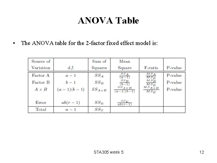
ANOVA Table • The ANOVA table for the 2 -factor fixed effect model is: STA 305 week 5 12

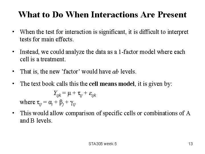
What to Do When Interactions Are Present • When the test for interaction is significant, it is difficult to interpret tests for main effects. • Instead, we could analyze the data as a 1 -factor model where each cell is a treatment. • That is, the new ’factor’ would have ab levels. • The text book calls this the cell means model, it is given by: Yijk = μ + τij + εijk where τij = αi + βj + γij • This would allow comparison of specific cells or combinations of A and B levels. STA 305 week 5 13

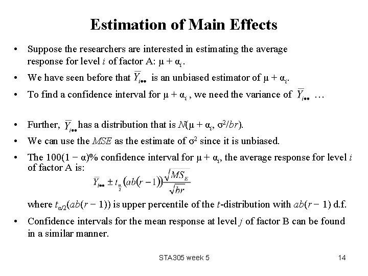
Estimation of Main Effects • Suppose the researchers are interested in estimating the average response for level i of factor A: μ + αi. • We have seen before that is an unbiased estimator of μ + αi. • To find a confidence interval for μ + αi , we need the variance of • Further, … has a distribution that is N(μ + αi, σ2/br). • We can use the MSE as the estimate of σ2 since it is unbiased. • The 100(1 − α)% confidence interval for μ + αi, the average response for level i of factor A is: where tα/2(ab(r − 1)) is upper percentile of the t-distribution with ab(r − 1) d. f. • Confidence intervals for the mean response at level j of factor B can be found in a similar manner. STA 305 week 5 14

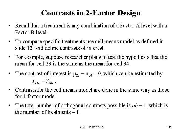
Contrasts in 2 -Factor Design • Recall that a treatment is any combination of a Factor A level with a Factor B level. • To compare specific treatments use cell means model as defined in slide 13, and define contrasts of interest. • For example, suppose researcher plans to test the hypothesis that the mean for cell 23 is the same as the mean for cell 34. • The contrast of interest is μ 23 − μ 34 = 0, which can be estimated by • Contrasts for the cell means model are done in the same way as those for 1 -factor model. • The total number of orthogonal contrasts possible is ab − 1, which is the number of treatments – 1. STA 305 week 5 15

• Generally, we write contrast and test it as follows… STA 305 week 5 16

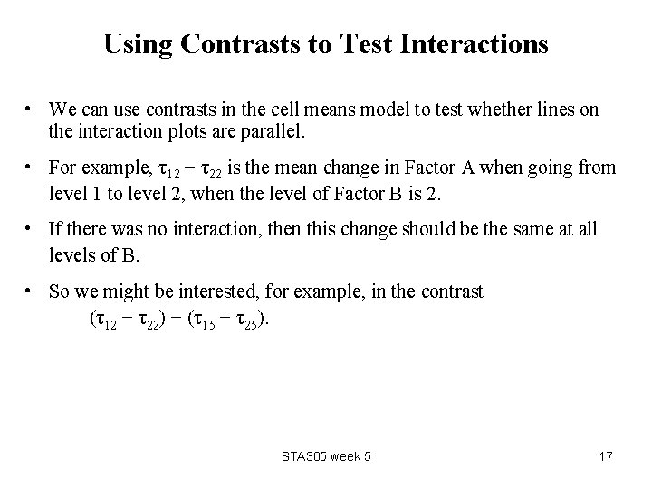
Using Contrasts to Test Interactions • We can use contrasts in the cell means model to test whether lines on the interaction plots are parallel. • For example, τ12 − τ22 is the mean change in Factor A when going from level 1 to level 2, when the level of Factor B is 2. • If there was no interaction, then this change should be the same at all levels of B. • So we might be interested, for example, in the contrast (τ12 − τ22) − (τ15 − τ25). STA 305 week 5 17

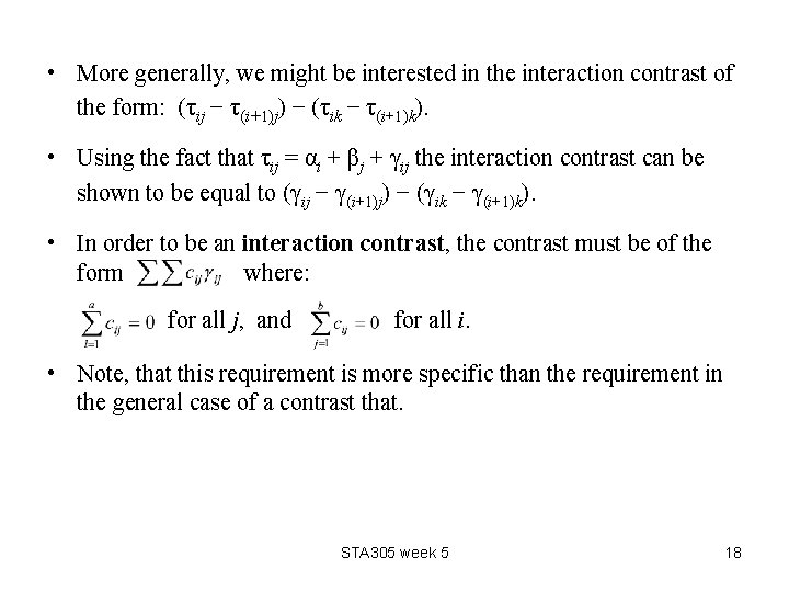
• More generally, we might be interested in the interaction contrast of the form: (τij − τ(i+1)j) − (τik − τ(i+1)k). • Using the fact that τij = αi + βj + γij the interaction contrast can be shown to be equal to (γij − γ(i+1)j) − (γik − γ(i+1)k). • In order to be an interaction contrast, the contrast must be of the form where: for all j, and for all i. • Note, that this requirement is more specific than the requirement in the general case of a contrast that. STA 305 week 5 18

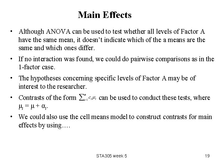
Main Effects • Although ANOVA can be used to test whether all levels of Factor A have the same mean, it doesn’t indicate which of the a means are the same and which ones differ. • If no interaction was found, we could do pairwise comparisons as in the 1 -factor case. • The hypotheses concerning specific levels of Factor A may be of interest to the researcher. • Contrasts of the form μi = μ + α i. can be used to conduct these tests, where • We could also use the cell means model to construct contrasts for main effects by using…. STA 305 week 5 19

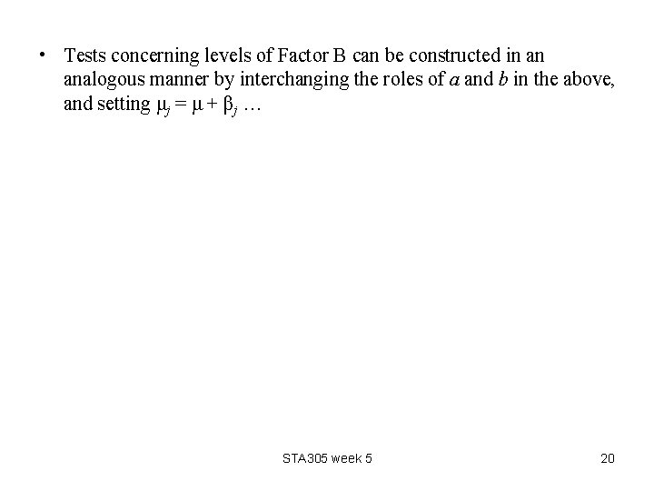
• Tests concerning levels of Factor B can be constructed in an analogous manner by interchanging the roles of a and b in the above, and setting μj = μ + βj … STA 305 week 5 20

Examples of Two-Factor Design • Two examples below illustrate some aspects of analysis of two-factor design. • In both cases, equal number of experimental units was randomly allocated to each combination of factor levels. • The designs are similar, but there are differences in the hypotheses of interest, and the steps taken in analysis. • In the first example (slide 22) interaction is found not to be significant, so tests concerning main effects can be made using ANOVA. • In the second example interactions are significant, and cells means model is used to compare treatments of interest. STA 305 week 5 21

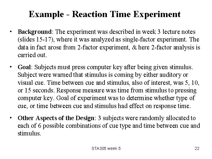
Example - Reaction Time Experiment • Background: The experiment was described in week 3 lecture notes (slides 15 -17), where it was analyzed as single-factor experiment. The data in fact arose from 2 -factor experiment, & here 2 -factor analysis is carried out. • Goal: Subjects must press computer key after being given stimulus. Subject were warned that stimulus is coming by either auditory or visual cue. Time between cue and stimulus, also of interest, was 5, 10, or 15 seconds. Response measure was time from stimulus to pressing computer key. Goal of experiment was to determine whether type of cue, or time between cue and stimulus had effect on response time. • Other Aspects of the Design: 3 subjects were randomly allocated to each of 6 possible combinations of cue type and time between cue and stimulus. STA 305 week 5 22

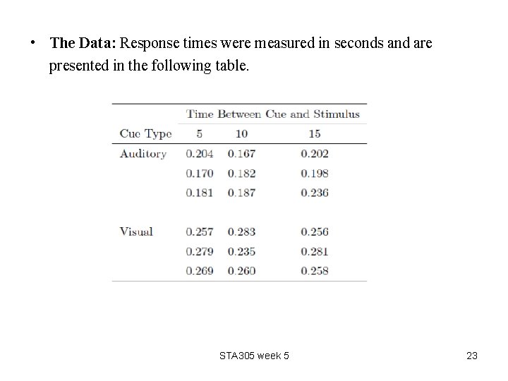
• The Data: Response times were measured in seconds and are presented in the following table. STA 305 week 5 23

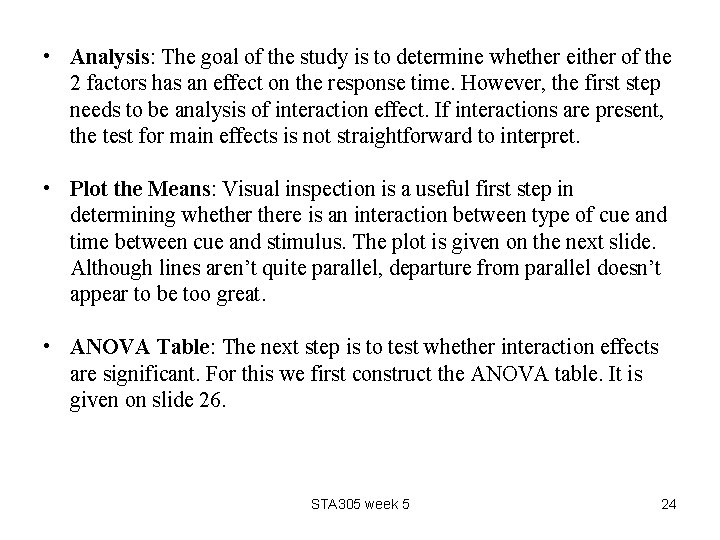
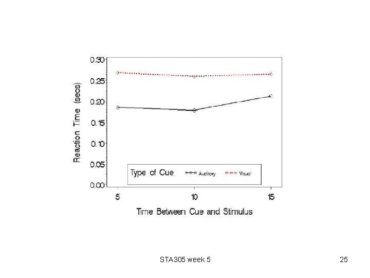
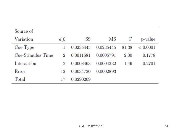
• Analysis: The goal of the study is to determine whether either of the 2 factors has an effect on the response time. However, the first step needs to be analysis of interaction effect. If interactions are present, the test for main effects is not straightforward to interpret. • Plot the Means: Visual inspection is a useful first step in determining whethere is an interaction between type of cue and time between cue and stimulus. The plot is given on the next slide. Although lines aren’t quite parallel, departure from parallel doesn’t appear to be too great. • ANOVA Table: The next step is to test whether interaction effects are significant. For this we first construct the ANOVA table. It is given on slide 26. STA 305 week 5 24

STA 305 week 5 25

STA 305 week 5 26

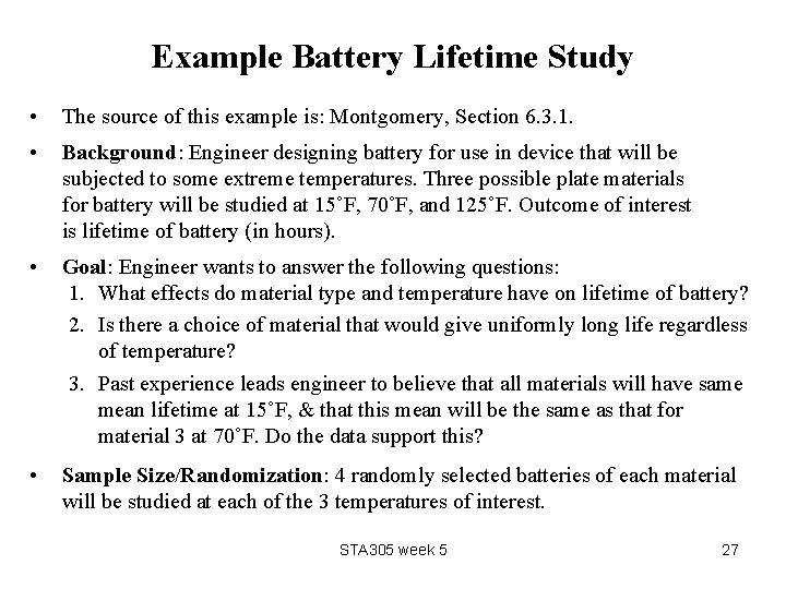
Example Battery Lifetime Study • The source of this example is: Montgomery, Section 6. 3. 1. • Background: Engineer designing battery for use in device that will be subjected to some extreme temperatures. Three possible plate materials for battery will be studied at 15˚F, 70˚F, and 125˚F. Outcome of interest is lifetime of battery (in hours). • Goal: Engineer wants to answer the following questions: 1. What effects do material type and temperature have on lifetime of battery? 2. Is there a choice of material that would give uniformly long life regardless of temperature? 3. Past experience leads engineer to believe that all materials will have same mean lifetime at 15˚F, & that this mean will be the same as that for material 3 at 70˚F. Do the data support this? • Sample Size/Randomization: 4 randomly selected batteries of each material will be studied at each of the 3 temperatures of interest. STA 305 week 5 27

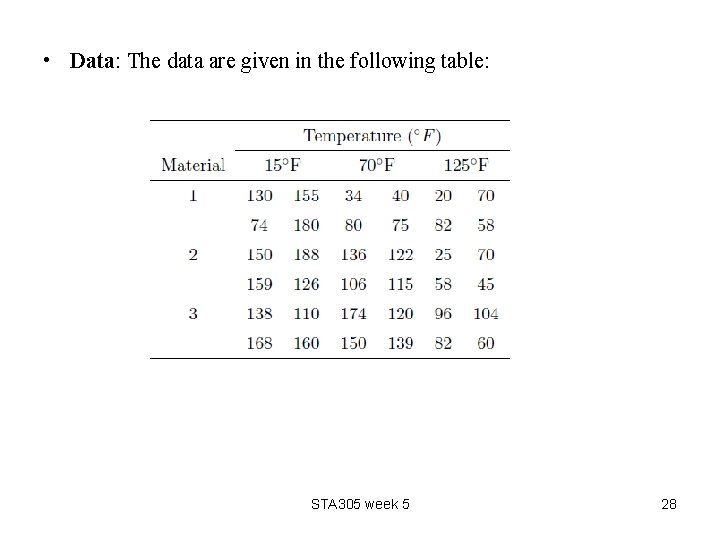
• Data: The data are given in the following table: STA 305 week 5 28

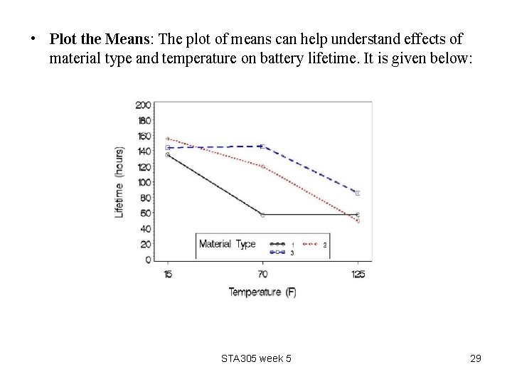
• Plot the Means: The plot of means can help understand effects of material type and temperature on battery lifetime. It is given below: STA 305 week 5 29

• From the plot it appears to be large interaction between material and temperature. • Generally, lifetimes are longest at lowest temperature for all materials. • Changing from low to intermediate temperature, battery life with material 3 increases, while it decreases for materials 1 and 2. • From intermediate to high temperature, mean lifetime decreases for materials 2 and 3 but is unchanged for material 1. • Material 3 seems to give the best results in terms of consistent lifetimes across temperatures. STA 305 week 5 30

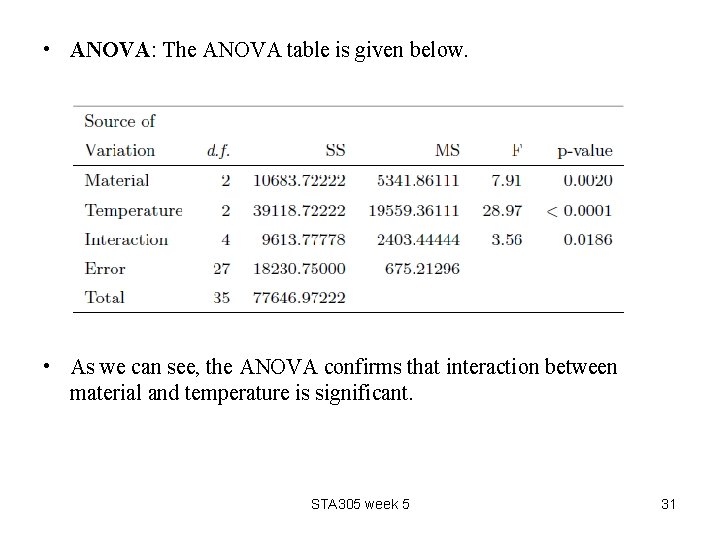
• ANOVA: The ANOVA table is given below. • As we can see, the ANOVA confirms that interaction between material and temperature is significant. STA 305 week 5 31

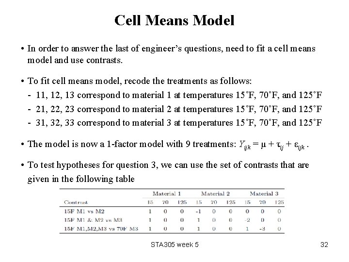
Cell Means Model • In order to answer the last of engineer’s questions, need to fit a cell means model and use contrasts. • To fit cell means model, recode the treatments as follows: - 11, 12, 13 correspond to material 1 at temperatures 15˚F, 70˚F, and 125˚F - 21, 22, 23 correspond to material 2 at temperatures 15˚F, 70˚F, and 125˚F - 31, 32, 33 correspond to material 3 at temperatures 15˚F, 70˚F, and 125˚F • The model is now a 1 -factor model with 9 treatments: Yijk = μ + τij + εijk. • To test hypotheses for question 3, we can use the set of contrasts that are given in the following table STA 305 week 5 32

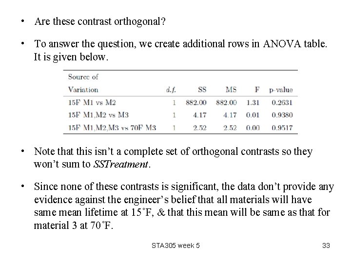
• Are these contrast orthogonal? • To answer the question, we create additional rows in ANOVA table. It is given below. • Note that this isn’t a complete set of orthogonal contrasts so they won’t sum to SSTreatment. • Since none of these contrasts is significant, the data don’t provide any evidence against the engineer’s belief that all materials will have same mean lifetime at 15˚F, & that this mean will be same as that for material 3 at 70˚F. STA 305 week 5 33

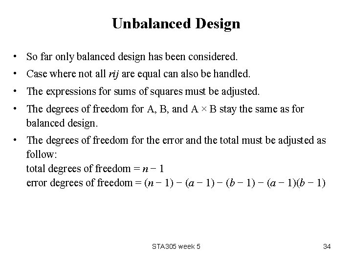
Unbalanced Design • So far only balanced design has been considered. • Case where not all rij are equal can also be handled. • The expressions for sums of squares must be adjusted. • The degrees of freedom for A, B, and A × B stay the same as for balanced design. • The degrees of freedom for the error and the total must be adjusted as follow: total degrees of freedom = n − 1 error degrees of freedom = (n − 1) − (a − 1) − (b − 1) − (a − 1)(b − 1) STA 305 week 5 34

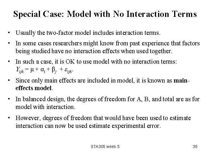
Special Case: Model with No Interaction Terms • Usually the two-factor model includes interaction terms. • In some cases researchers might know from past experience that factors being studied have no interaction effects when used together. • In such a case, it is OK to use model with no interaction terms: Yijk = μ + αi + βj + εijk. • Since only main effects are included in model, it is known as maineffects model. • In balanced design, the degrees of freedom for A, B, and total are as for model with interaction. • However, degrees of freedom that would have been used to estimate interaction can now be used estimate experimental error. STA 305 week 5 35

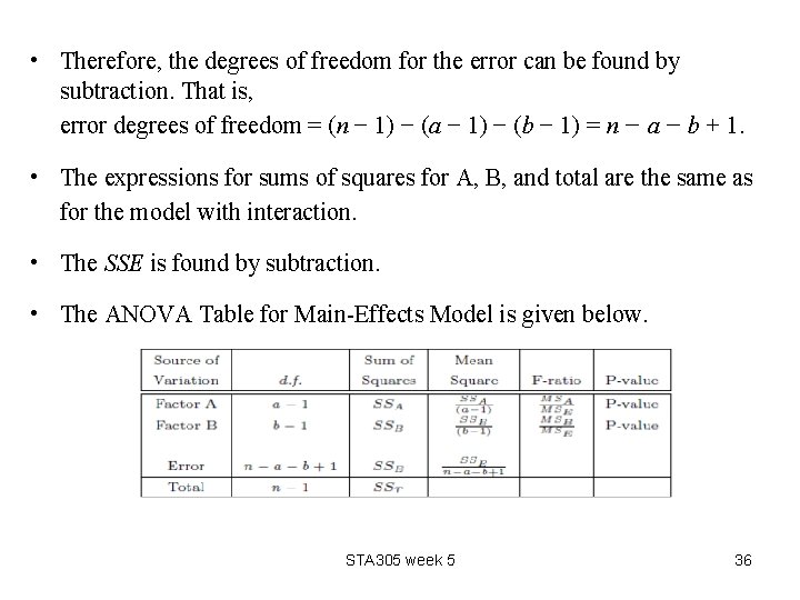
• Therefore, the degrees of freedom for the error can be found by subtraction. That is, error degrees of freedom = (n − 1) − (a − 1) − (b − 1) = n − a − b + 1. • The expressions for sums of squares for A, B, and total are the same as for the model with interaction. • The SSE is found by subtraction. • The ANOVA Table for Main-Effects Model is given below. STA 305 week 5 36

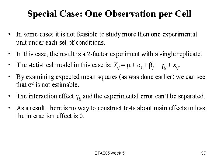
Special Case: One Observation per Cell • In some cases it is not feasible to study more then one experimental unit under each set of conditions. • In this case, the result is a 2 -factor experiment with a single replicate. • The statistical model in this case is: Yij = μ + αi + βj + γij + εij. • By examining expected mean squares (as was done earlier) we can see that σ2 is not estimable. • The interaction effect γij and the experimental error can’t be separated. • As a result, there is no way to construct tests about main effects unless the interaction effect is 0. STA 305 week 5 37

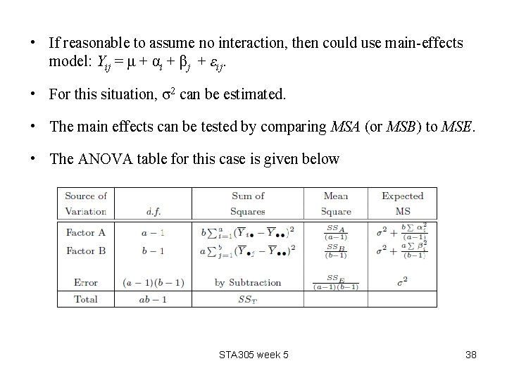
• If reasonable to assume no interaction, then could use main-effects model: Yij = μ + αi + βj + εij. • For this situation, σ2 can be estimated. • The main effects can be tested by comparing MSA (or MSB) to MSE. • The ANOVA table for this case is given below STA 305 week 5 38

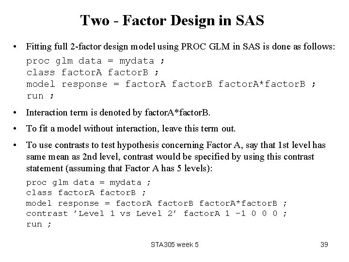
Two - Factor Design in SAS • Fitting full 2 -factor design model using PROC GLM in SAS is done as follows: proc glm data = mydata ; class factor. A factor. B ; model response = factor. A factor. B factor. A*factor. B ; run ; • Interaction term is denoted by factor. A*factor. B. • To fit a model without interaction, leave this term out. • To use contrasts to test hypothesis concerning Factor A, say that 1 st level has same mean as 2 nd level, contrast would be specified by using this contrast statement (assuming that Factor A has 5 levels): proc glm data = mydata ; class factor. A factor. B ; model response = factor. A factor. B factor. A*factor. B ; contrast ’Level 1 vs Level 2’ factor. A 1 -1 0 0 0 ; run ; STA 305 week 5 39

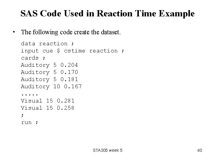
SAS Code Used in Reaction Time Example • The following code create the dataset. data reaction ; input cue $ cstime reaction ; cards ; Auditory 5 0. 204 Auditory 5 0. 170 Auditory 5 0. 181 Auditory 10 0. 167. . . Visual 15 0. 281 Visual 15 0. 258 ; run ; STA 305 week 5 40

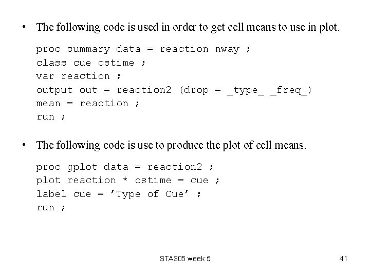
• The following code is used in order to get cell means to use in plot. proc summary data = reaction nway ; class cue cstime ; var reaction ; output out = reaction 2 (drop = _type_ _freq_) mean = reaction ; run ; • The following code is use to produce the plot of cell means. proc gplot data = reaction 2 ; plot reaction * cstime = cue ; label cue = ’Type of Cue’ ; run ; STA 305 week 5 41

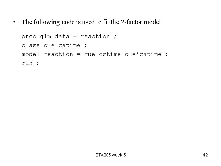
• The following code is used to fit the 2 -factor model. proc glm data = reaction ; class cue cstime ; model reaction = cue cstime cue*cstime ; run ; STA 305 week 5 42

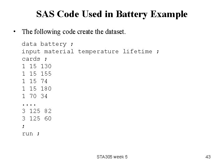
SAS Code Used in Battery Example • The following code create the dataset. data battery ; input material temperature lifetime ; cards ; 1 15 130 1 15 155 1 15 74 1 15 180 1 70 34. . 3 125 82 3 125 60 ; run ; STA 305 week 5 43

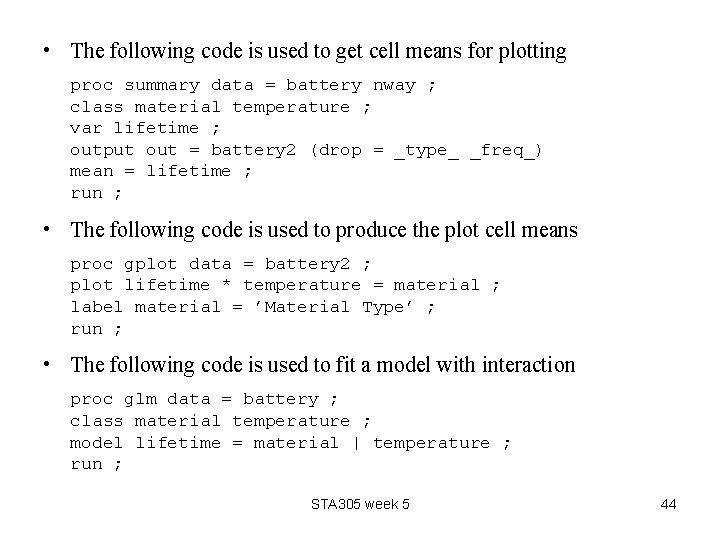
• The following code is used to get cell means for plotting proc summary data = battery nway ; class material temperature ; var lifetime ; output out = battery 2 (drop = _type_ _freq_) mean = lifetime ; run ; • The following code is used to produce the plot cell means proc gplot data = battery 2 ; plot lifetime * temperature = material ; label material = ’Material Type’ ; run ; • The following code is used to fit a model with interaction proc glm data = battery ; class material temperature ; model lifetime = material | temperature ; run ; STA 305 week 5 44

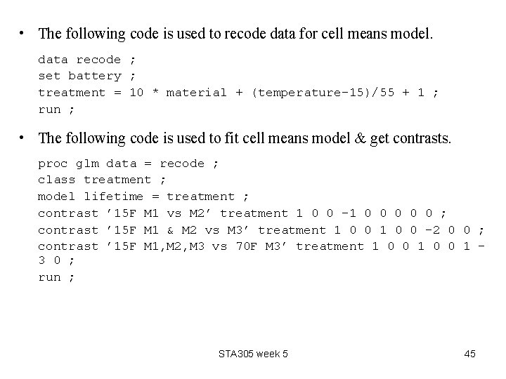
• The following code is used to recode data for cell means model. data recode ; set battery ; treatment = 10 * material + (temperature-15)/55 + 1 ; run ; • The following code is used to fit cell means model & get contrasts. proc glm data = recode ; class treatment ; model lifetime = treatment ; contrast ’ 15 F M 1 vs M 2’ treatment 1 0 0 -1 0 0 0 ; contrast ’ 15 F M 1 & M 2 vs M 3’ treatment 1 0 0 -2 0 0 ; contrast ’ 15 F M 1, M 2, M 3 vs 70 F M 3’ treatment 1 0 0 1 3 0 ; run ; STA 305 week 5 45