Two developments in discovery tests use of weighted

Two developments in discovery tests: use of weighted Monte Carlo events and an improved measure of experimental sensitivity Progress on Statistical Issues in Searches SLAC, 4 -6 June, 2012 Glen Cowan Physics Department Royal Holloway, University of London www. pp. rhul. ac. uk/~cowan g. cowan@rhul. ac. uk G. Cowan SLAC Statistics Meeting / 4 -6 June 2012 / Two Developments 1

Outline Two issues of practical importance in recent LHC analyses: 1) In many searches for new signal processes, estimates of rates of some background components often based on Monte Carlo with weighted events. Some care (and assumptions) are required to assess the effect of the finite MC sample on the result of the test. 2) A measure of discovery sensitivity is often used to plan a future analysis, e. g. , s/√b, gives approximate expected discovery significance (test of s = 0) when counting n ~ Poisson(s+b). A measure of discovery significance is proposed that takes into account uncertainty in the background rate. G. Cowan SLAC Statistics Meeting / 4 -6 June 2012 / Two Developments 2

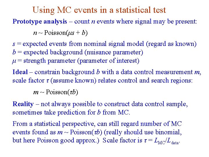
Using MC events in a statistical test Prototype analysis – count n events where signal may be present: n ~ Poisson(μs + b) s = expected events from nominal signal model (regard as known) b = expected background (nuisance parameter) μ = strength parameter (parameter of interest) Ideal – constrain background b with a data control measurement m, scale factor τ (assume known) relates control and search regions: m ~ Poisson(τb) Reality – not always possible to construct data control sample, sometimes take prediction for b from MC. From a statistical perspective, can still regard number of MC events found as m ~ Poisson(τb) (really should use binomial, but here Poisson good approx. ) Scale factor is τ = LMC/Ldata. G. Cowan SLAC Statistics Meeting / 4 -6 June 2012 / Two Developments 3

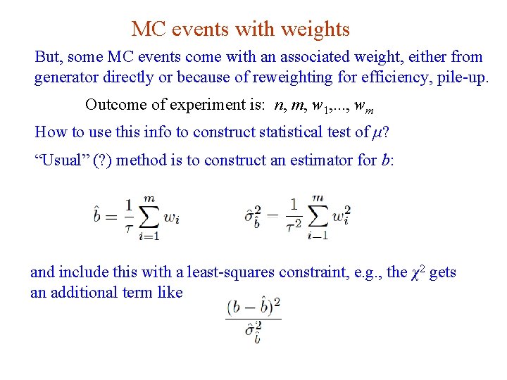
MC events with weights But, some MC events come with an associated weight, either from generator directly or because of reweighting for efficiency, pile-up. Outcome of experiment is: n, m, w 1, . . . , wm How to use this info to construct statistical test of μ? “Usual” (? ) method is to construct an estimator for b: and include this with a least-squares constraint, e. g. , the χ2 gets an additional term like G. Cowan SLAC Statistics Meeting / 4 -6 June 2012 / Two Developments 4

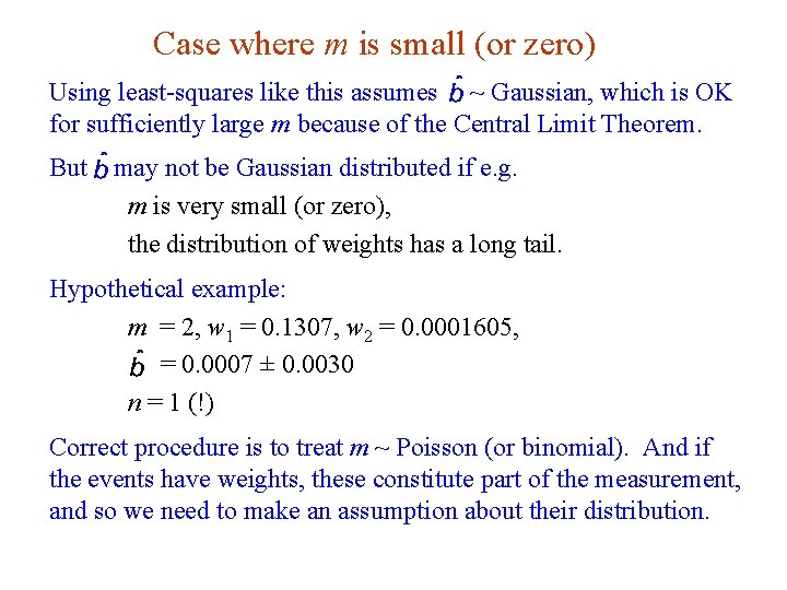
Case where m is small (or zero) Using least-squares like this assumes ~ Gaussian, which is OK for sufficiently large m because of the Central Limit Theorem. But may not be Gaussian distributed if e. g. m is very small (or zero), the distribution of weights has a long tail. Hypothetical example: m = 2, w 1 = 0. 1307, w 2 = 0. 0001605, = 0. 0007 ± 0. 0030 n = 1 (!) Correct procedure is to treat m ~ Poisson (or binomial). And if the events have weights, these constitute part of the measurement, and so we need to make an assumption about their distribution. G. Cowan SLAC Statistics Meeting / 4 -6 June 2012 / Two Developments 5

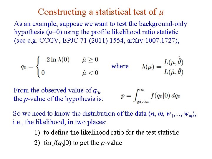
Constructing a statistical test of μ As an example, suppose we want to test the background-only hypothesis (μ=0) using the profile likelihood ratio statistic (see e. g. CCGV, EPJC 71 (2011) 1554, ar. Xiv: 1007. 1727), where From the observed value of q 0, the p-value of the hypothesis is: So we need to know the distribution of the data (n, m, w 1, . . . , wm), i. e. , the likelihood, in two places: 1) to define the likelihood ratio for the test statistic 2) for f(q 0|0) to get the p-value G. Cowan SLAC Statistics Meeting / 4 -6 June 2012 / Two Developments 6

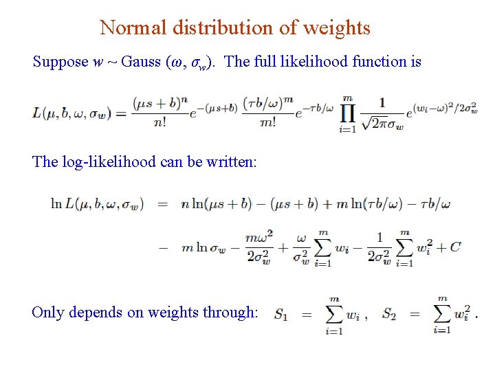
Normal distribution of weights Suppose w ~ Gauss (ω, σw). The full likelihood function is The log-likelihood can be written: Only depends on weights through: G. Cowan SLAC Statistics Meeting / 4 -6 June 2012 / Two Developments 7

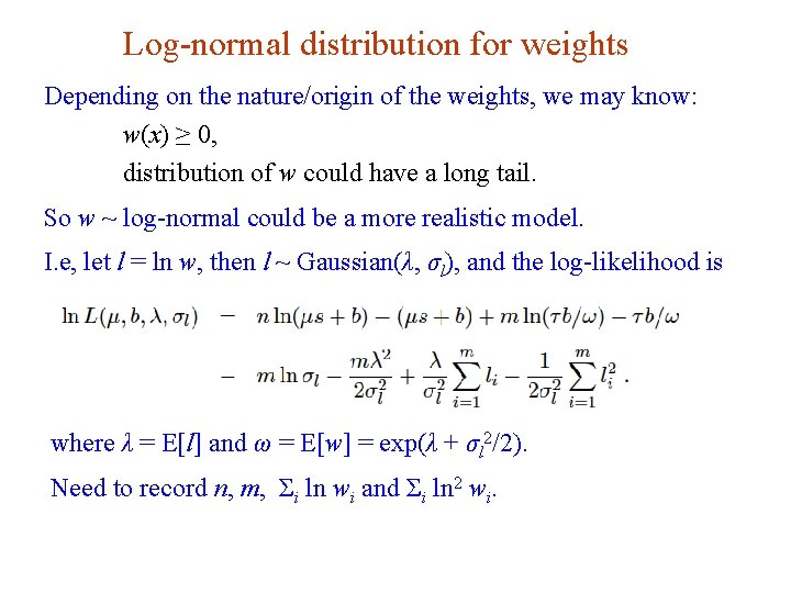
Log-normal distribution for weights Depending on the nature/origin of the weights, we may know: w(x) ≥ 0, distribution of w could have a long tail. So w ~ log-normal could be a more realistic model. I. e, let l = ln w, then l ~ Gaussian(λ, σl), and the log-likelihood is where λ = E[l] and ω = E[w] = exp(λ + σl 2/2). Need to record n, m, Σi ln wi and Σi ln 2 wi. G. Cowan SLAC Statistics Meeting / 4 -6 June 2012 / Two Developments 8

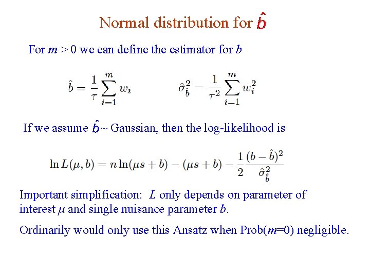
Normal distribution for For m > 0 we can define the estimator for b If we assume ~ Gaussian, then the log-likelihood is Important simplification: L only depends on parameter of interest μ and single nuisance parameter b. Ordinarily would only use this Ansatz when Prob(m=0) negligible. G. Cowan SLAC Statistics Meeting / 4 -6 June 2012 / Two Developments 9

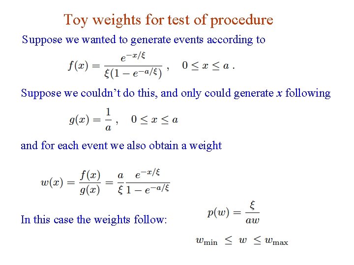
Toy weights for test of procedure Suppose we wanted to generate events according to Suppose we couldn’t do this, and only could generate x following and for each event we also obtain a weight In this case the weights follow: G. Cowan SLAC Statistics Meeting / 4 -6 June 2012 / Two Developments 10

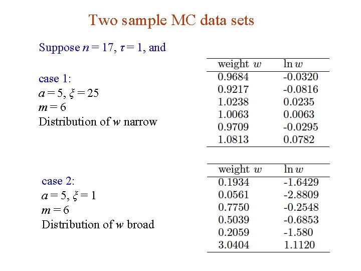
Two sample MC data sets Suppose n = 17, τ = 1, and case 1: a = 5, ξ = 25 m=6 Distribution of w narrow case 2: a = 5, ξ = 1 m=6 Distribution of w broad G. Cowan SLAC Statistics Meeting / 4 -6 June 2012 / Two Developments 11

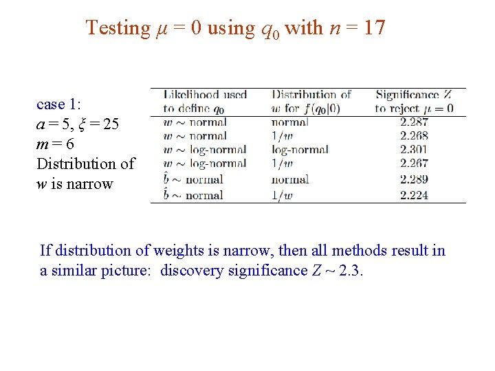
Testing μ = 0 using q 0 with n = 17 case 1: a = 5, ξ = 25 m=6 Distribution of w is narrow If distribution of weights is narrow, then all methods result in a similar picture: discovery significance Z ~ 2. 3. G. Cowan SLAC Statistics Meeting / 4 -6 June 2012 / Two Developments 12

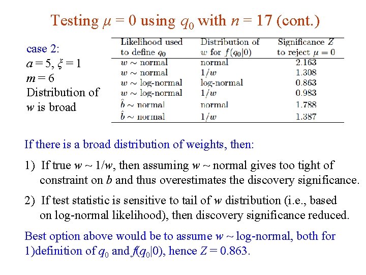
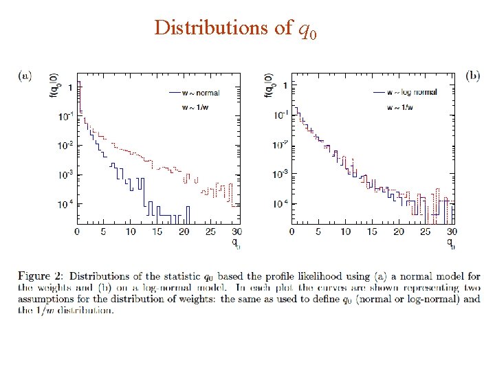
Testing μ = 0 using q 0 with n = 17 (cont. ) case 2: a = 5, ξ = 1 m=6 Distribution of w is broad If there is a broad distribution of weights, then: 1) If true w ~ 1/w, then assuming w ~ normal gives too tight of constraint on b and thus overestimates the discovery significance. 2) If test statistic is sensitive to tail of w distribution (i. e. , based on log-normal likelihood), then discovery significance reduced. Best option above would be to assume w ~ log-normal, both for 1)definition of q 0 and f(q 0|0), hence Z = 0. 863. G. Cowan SLAC Statistics Meeting / 4 -6 June 2012 / Two Developments 13

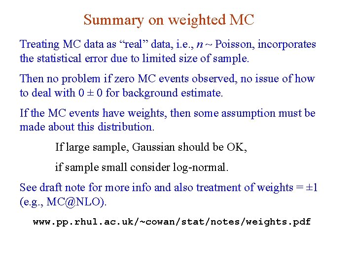
Summary on weighted MC Treating MC data as “real” data, i. e. , n ~ Poisson, incorporates the statistical error due to limited size of sample. Then no problem if zero MC events observed, no issue of how to deal with 0 ± 0 for background estimate. If the MC events have weights, then some assumption must be made about this distribution. If large sample, Gaussian should be OK, if sample small consider log-normal. See draft note for more info and also treatment of weights = ± 1 (e. g. , MC@NLO). www. pp. rhul. ac. uk/~cowan/stat/notes/weights. pdf G. Cowan SLAC Statistics Meeting / 4 -6 June 2012 / Two Developments 14

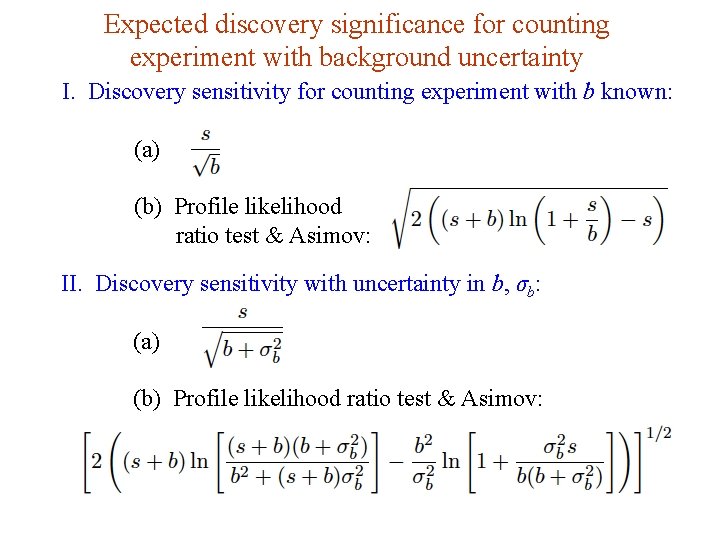
Expected discovery significance for counting experiment with background uncertainty I. Discovery sensitivity for counting experiment with b known: (a) (b) Profile likelihood ratio test & Asimov: II. Discovery sensitivity with uncertainty in b, σb: (a) (b) Profile likelihood ratio test & Asimov: G. Cowan SLAC Statistics Meeting / 4 -6 June 2012 / Two Developments 15

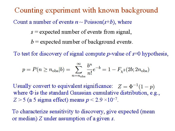
Counting experiment with known background Count a number of events n ~ Poisson(s+b), where s = expected number of events from signal, b = expected number of background events. To test for discovery of signal compute p-value of s=0 hypothesis, Usually convert to equivalent significance: where Φ is the standard Gaussian cumulative distribution, e. g. , Z > 5 (a 5 sigma effect) means p < 2. 9 × 10 -7. To characterize sensitivity to discovery, give expected (mean or median) Z under assumption of a given s. G. Cowan SLAC Statistics Meeting / 4 -6 June 2012 / Two Developments 16

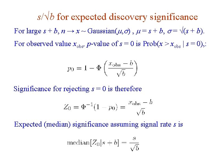
s/√b for expected discovery significance For large s + b, n → x ~ Gaussian(m, s) , m = s + b, s = √(s + b). For observed value xobs, p-value of s = 0 is Prob(x > xobs | s = 0), : Significance for rejecting s = 0 is therefore Expected (median) significance assuming signal rate s is G. Cowan SLAC Statistics Meeting / 4 -6 June 2012 / Two Developments 17

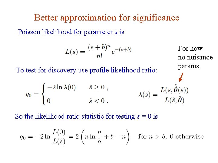
Better approximation for significance Poisson likelihood for parameter s is To test for discovery use profile likelihood ratio: For now no nuisance params. So the likelihood ratio statistic for testing s = 0 is G. Cowan SLAC Statistics Meeting / 4 -6 June 2012 / Two Developments 18

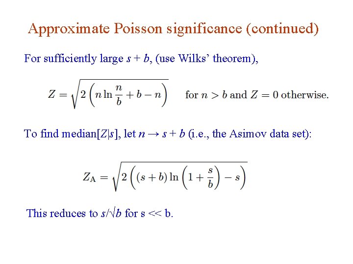
Approximate Poisson significance (continued) For sufficiently large s + b, (use Wilks’ theorem), To find median[Z|s], let n → s + b (i. e. , the Asimov data set): This reduces to s/√b for s << b. G. Cowan SLAC Statistics Meeting / 4 -6 June 2012 / Two Developments 19

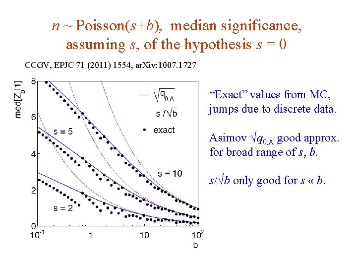
n ~ Poisson(s+b), median significance, assuming s, of the hypothesis s = 0 CCGV, EPJC 71 (2011) 1554, ar. Xiv: 1007. 1727 “Exact” values from MC, jumps due to discrete data. Asimov √q 0, A good approx. for broad range of s, b. s/√b only good for s « b. G. Cowan SLAC Statistics Meeting / 4 -6 June 2012 / Two Developments 20

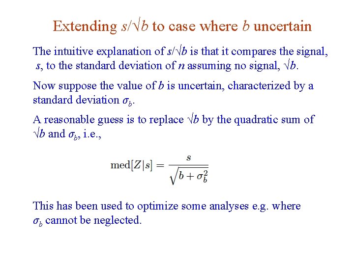
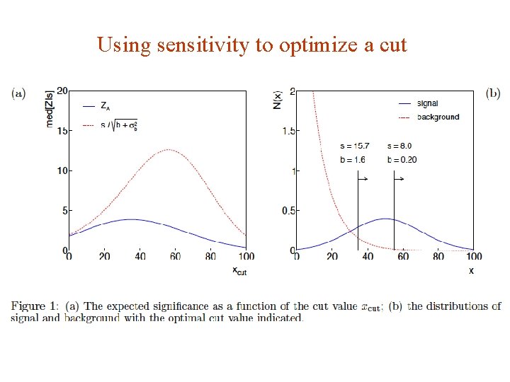
Extending s/√b to case where b uncertain The intuitive explanation of s/√b is that it compares the signal, s, to the standard deviation of n assuming no signal, √b. Now suppose the value of b is uncertain, characterized by a standard deviation σb. A reasonable guess is to replace √b by the quadratic sum of √b and σb, i. e. , This has been used to optimize some analyses e. g. where σb cannot be neglected. G. Cowan SLAC Statistics Meeting / 4 -6 June 2012 / Two Developments 21

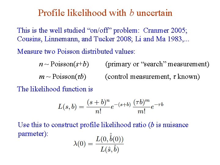
Profile likelihood with b uncertain This is the well studied “on/off” problem: Cranmer 2005; Cousins, Linnemann, and Tucker 2008; Li and Ma 1983, . . . Measure two Poisson distributed values: n ~ Poisson(s+b) (primary or “search” measurement) m ~ Poisson(τb) (control measurement, τ known) The likelihood function is Use this to construct profile likelihood ratio (b is nuisance parmeter): G. Cowan SLAC Statistics Meeting / 4 -6 June 2012 / Two Developments 22

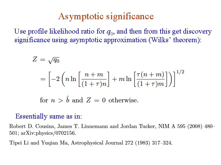
Asymptotic significance Use profile likelihood ratio for q 0, and then from this get discovery significance using asymptotic approximation (Wilks’ theorem): Essentially same as in: G. Cowan SLAC Statistics Meeting / 4 -6 June 2012 / Two Developments 23

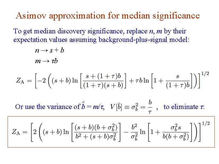
Asimov approximation for median significance To get median discovery significance, replace n, m by their expectation values assuming background-plus-signal model: n→s+b m → τb Or use the variance of ˆb = m/τ, G. Cowan , to eliminate τ: SLAC Statistics Meeting / 4 -6 June 2012 / Two Developments 24

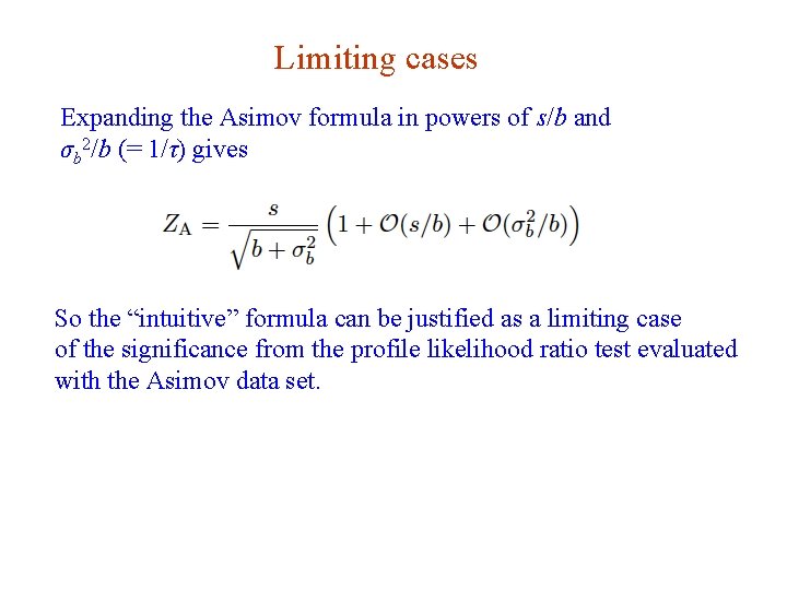
Limiting cases Expanding the Asimov formula in powers of s/b and σb 2/b (= 1/τ) gives So the “intuitive” formula can be justified as a limiting case of the significance from the profile likelihood ratio test evaluated with the Asimov data set. G. Cowan SLAC Statistics Meeting / 4 -6 June 2012 / Two Developments 25

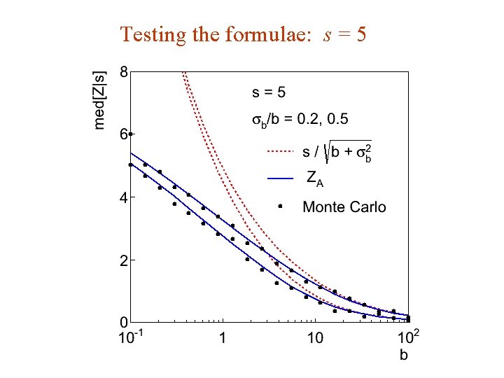
Testing the formulae: s = 5 G. Cowan SLAC Statistics Meeting / 4 -6 June 2012 / Two Developments 26

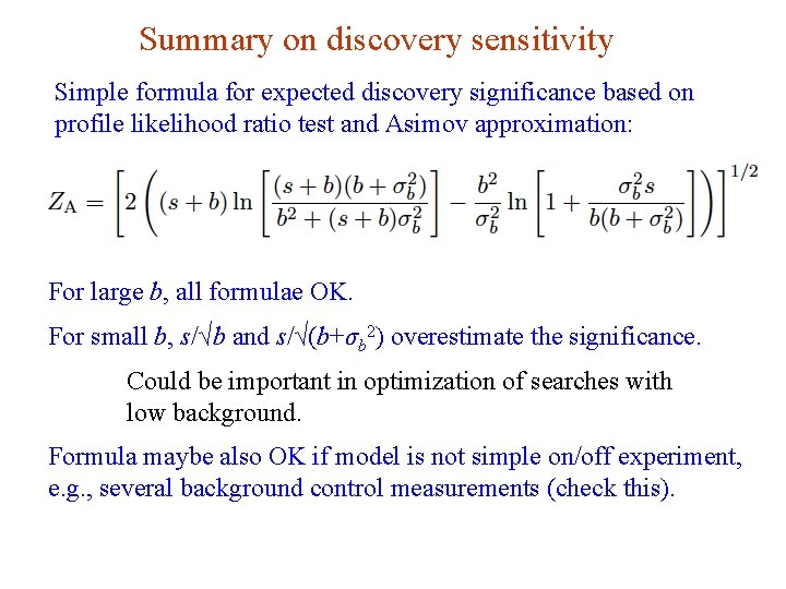
Summary on discovery sensitivity Simple formula for expected discovery significance based on profile likelihood ratio test and Asimov approximation: For large b, all formulae OK. For small b, s/√b and s/√(b+σb 2) overestimate the significance. Could be important in optimization of searches with low background. Formula maybe also OK if model is not simple on/off experiment, e. g. , several background control measurements (check this). G. Cowan SLAC Statistics Meeting / 4 -6 June 2012 / Two Developments 27

Extra slides G. Cowan SLAC Statistics Meeting / 4 -6 June 2012 / Two Developments 28

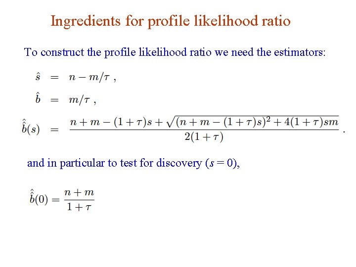
Ingredients for profile likelihood ratio To construct the profile likelihood ratio we need the estimators: and in particular to test for discovery (s = 0), G. Cowan SLAC Statistics Meeting / 4 -6 June 2012 / Two Developments 29

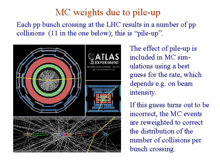
MC weights due to pile-up Each pp bunch crossing at the LHC results in a number of pp collisions (11 in the one below); this is “pile-up”. The effect of pile-up is included in MC simulations using a best guess for the rate, which depends e. g. on beam intensity. If this guess turns out to be incorrect, the MC events are reweighted to correct the distribution of the number of collisions per bunch crossing. G. Cowan SLAC Statistics Meeting / 4 -6 June 2012 / Two Developments 30

Using sensitivity to optimize a cut G. Cowan SLAC Statistics Meeting / 4 -6 June 2012 / Two Developments 31

Distributions of q 0 G. Cowan SLAC Statistics Meeting / 4 -6 June 2012 / Two Developments 32