Tutorial on General Equilibrium Analysis HeckscherOhlinSamuelson Trade Model

Tutorial on General Equilibrium Analysis: Heckscher-Ohlin-Samuelson Trade Model The Microeconomics of International Trade ECN 230 Roberto J. Garcia School of Economics and Business, NMBU Session 4

General equilibrium trade analysis II Heckscher-Ohlin-Samuelson (H-O-S) model Model specification and assumptions Specification • Two countries: North and South • Two goods: agricultural (A) and manufactured (M) • Two factors: labor (L) and capital (K) Assumptions • • Identical goods and factors Factor mobility across sectors not across borders Production functions are identical Factor endowments differ Factor intensity in production Competitive markets Resources fully employed; world production = consumption Preferences can be same or different 1

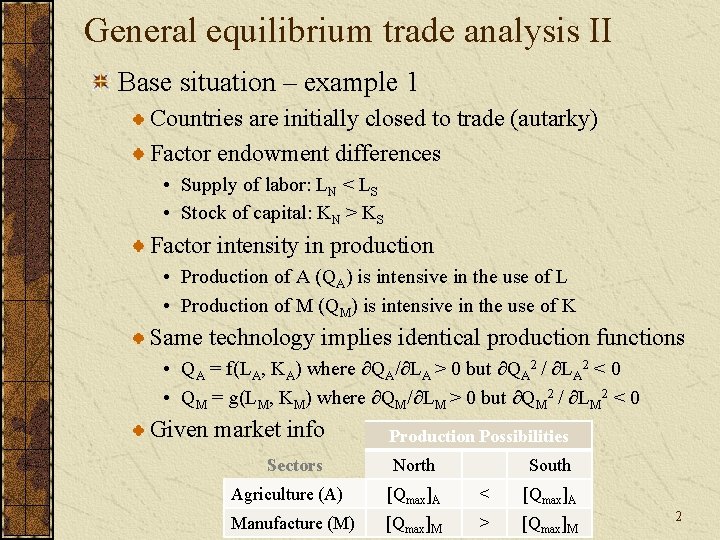
General equilibrium trade analysis II Base situation – example 1 Countries are initially closed to trade (autarky) Factor endowment differences • Supply of labor: LN < LS • Stock of capital: KN > KS Factor intensity in production • Production of A (QA) is intensive in the use of L • Production of M (QM) is intensive in the use of K Same technology implies identical production functions • QA = f(LA, KA) where ∂QA/∂LA > 0 but ∂QA 2 / ∂LA 2 < 0 • QM = g(LM, KM) where ∂QM/∂LM > 0 but ∂QM 2 / ∂LM 2 < 0 Given market info Sectors Production Possibilities North South Agriculture (A) [Qmax]A < [Qmax]A Manufacture (M) [Qmax]M > [Qmax]M 2

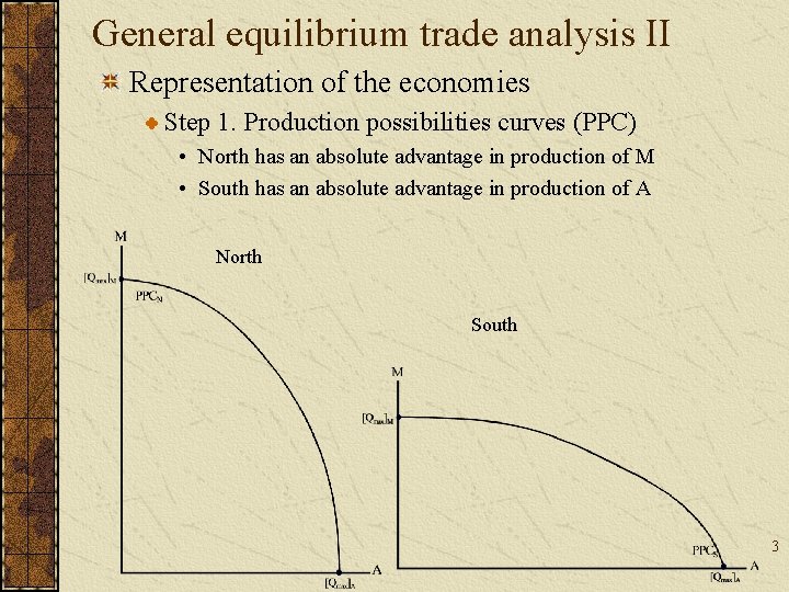
General equilibrium trade analysis II Representation of the economies Step 1. Production possibilities curves (PPC) • North has an absolute advantage in production of M • South has an absolute advantage in production of A North South 3

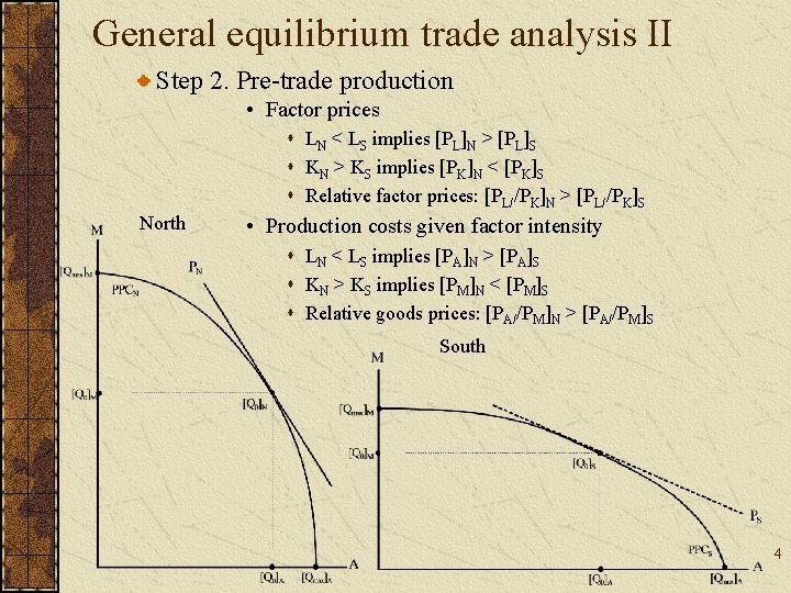
General equilibrium trade analysis II Step 2. Pre-trade production • Factor prices s LN < LS implies [PL]N > [PL]S s KN > KS implies [PK]N < [PK]S s Relative factor prices: [PL//PK]N > [PL//PK]S North • Production costs given factor intensity s LN < LS implies [PA]N > [PA]S s KN > KS implies [PM]N < [PM]S s Relative goods prices: [PA//PM]N > [PA//PM]S South 4

General equilibrium trade analysis II Step 3. Pre-trade consumption • Budget line is the consumption possibilities curve • Suppose preferences for the goods is given as shown below North s Utility maximization at tangency of SW and budget line s Optimal combination of A, M in consumption is at [Co], which includes [Co]A and [Co]M given prices and income South 5

General equilibrium trade analysis II General equilibrium, pre-trade situation in North • Closed economy: production equals consumption • [Qo] = [Co] implies [Qo]A = [Co]A and [Qo]M = [Co]M • [PA / PM]N = ∆M/∆A = slope of PPC = slope of SW = slope of budget line North Agricultural sector Manufacturing sector 6

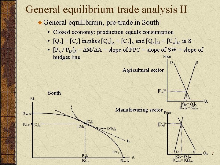
General equilibrium trade analysis II General equilibrium, pre-trade in South • Closed economy: production equals consumption • [Qo] = [Co] implies [Qo]A = [Co]A and [Qo]M = [Co]M in S • [PA / PM]S = ∆M/∆A = slope of PPC = slope of SW = slope of budget line Agricultural sector South Manufacturing sector 7

General equilibrium trade analysis II Partial equilibrium, pre-trade North South Agricultural sector [PA]N > [PA]S Manufacturing sector [PM]N < [PM]S [PA/PM]N > [PA/PM]S 8

General equilibrium trade analysis II Partial equilibrium, pre-trade North South Agricultural sector [PA]N > [PA]S Manufacturing sector [PM]N < [PM]S [PA/PM]N > [PA/PM]S 9

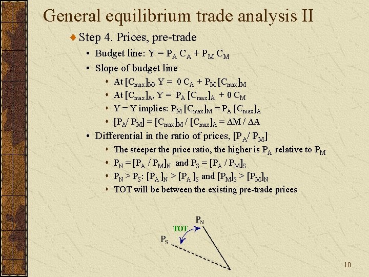
General equilibrium trade analysis II Step 4. Prices, pre-trade • Budget line: Y = PA CA + PM CM • Slope of budget line s s At [Cmax]M, Y = 0 CA + PM [Cmax]M At [Cmax]A, Y = PA [Cmax]A + 0 CM Y = Y implies: PM [Cmax]M = PA [Cmax]A [PA/ PM] = [Cmax]M / [Cmax]A = ∆M / ∆A • Differential in the ratio of prices, [PA/ PM] s s The steeper the price ratio, the higher is PA relative to PM PN = [PA / PM]N and PS = [PA / PM]S PN > PS: [PA ]N > [PA ]S and [PM]S > [PM]N TOT will be between the existing pre-trade prices 10

General equilibrium trade analysis II Step 5. World prices, TOT and the price changes • Prices in the agricultural sector • Prices in the manufacturing sector 11

General equilibrium trade analysis II • TOT is the ratio of world prices: [PA/PM]W • Price changes in North: [PA/PM]N > [PA/PM]W s ↓ PA from [PA]N to [PA]W s ↑ PM from [PM]N to [PM]W North 12

General equilibrium trade analysis II • Price changes in South: [PA/PM]S < [PA/PM]W s ↑ PA from [PA]S to [PA]W s ↓ PM from [PM]S to [PM]W South 13

General equilibrium trade analysis II • Trade triangles • TOT: [PA/PM]W = [QM/QA]T s Relative prices of A for M on the world market s The quantity of A that must be traded to get a unit of M North South 14

General equilibrium trade analysis II Step 6. Welfare implications • The change in prices from pre-trade to the terms of trade increases purchasing power in both countries (outward shift in CPC or budget line) and raises utility (SW) • The gains from trade results from the process of specialization and trade that improves efficiency and welfare s s Efficiency in resource allocation Efficiency in production Efficiency in consumption Efficiency in exchange 15

General equilibrium trade analysis II Concluding comments General lessons from the results • Price differentials create an incentive for trade • A cost-competitive country has a comparative advantage and will be a net exporting country in a free trade situation • A high-cost country has a comparative disadvantage and will be a net importing country in a free trade situation • Specialization and trade result in gains that represent efficiency in resource use, production, consumption and exchange • The optimal amount traded is determined by the TOT bringing all markets into equilibrium Limitations and weaknesses of the model • Trade based on factor endowment differences shifts focus of comparative advantage toward supply side factors • Demand-side matters are important and likely to play more of a role in trade in the future • The underlying assumptions are still important for the results 16