Tutorial Markov chain Monte Carlo Professor Zhu Han

Tutorial: Markov chain Monte Carlo Professor Zhu Han Department of Electrical Engineering University of Houston Thanks for Qiuyang Shen and Yan Zhu

Outline • Motivations • MCMC Algorithms • Applications • Conclusions Ref link @https: //www. azernews. az/oil_and_gas/127728. html. Photograph by Trend. 2

Outline • The motivations of Markov chain Monte Carlo • Bayesian Inference • MCMC sampling algorithms • • Bayesian inference and random-walk sampling Hybrid Monte Carlo Sampling Self-parameterizing method: trans-dimensional MCMC Accelerate Bayesian inference: tempering method • Applications • Statistical inference of earth resistivity model • Intermittent connectivity model in satellite links • Conclusion 3

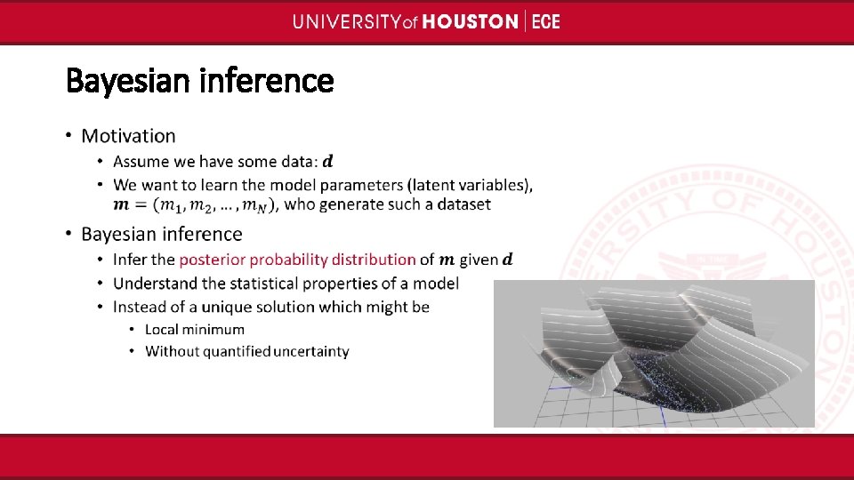
Bayesian inference •

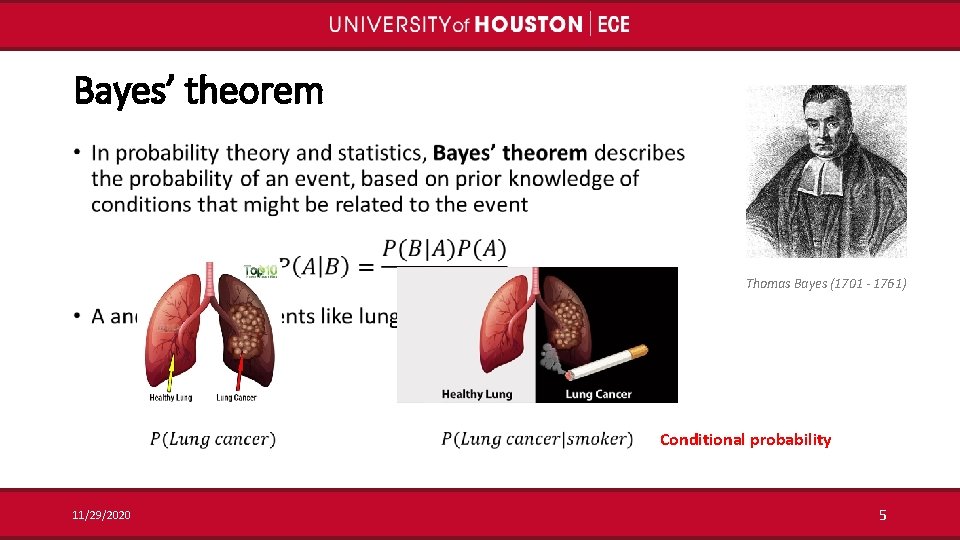
Bayes’ theorem • Thomas Bayes (1701 - 1761) 11/29/2020 Conditional probability 5

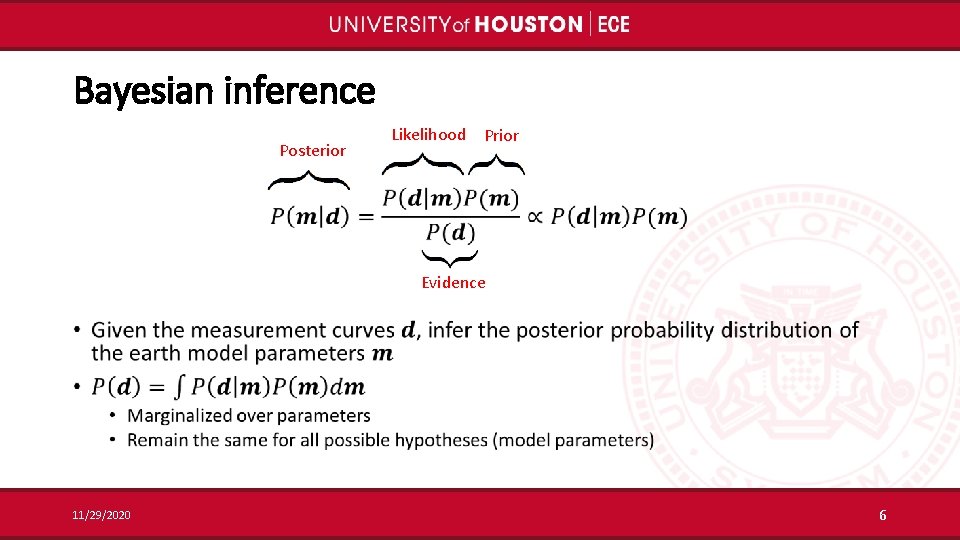
Bayesian inference • Posterior Likelihood Prior Evidence 11/29/2020 6

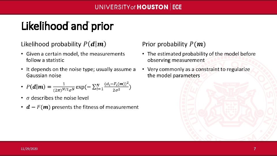
Likelihood and prior • 11/29/2020 • 7

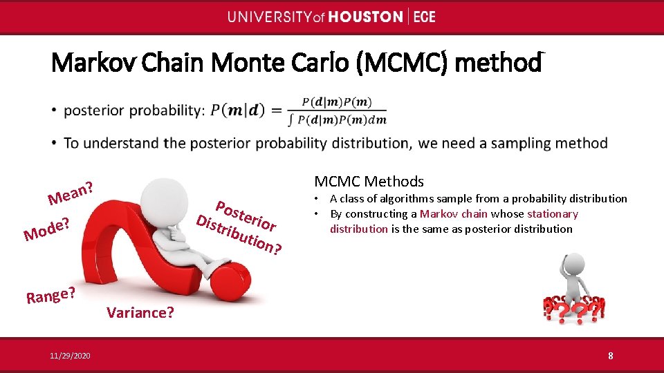
Markov Chain Monte Carlo (MCMC) method • MCMC Methods ean? M Pos Dist terior ribu tion ? e? d o M Range? 11/29/2020 • A class of algorithms sample from a probability distribution • By constructing a Markov chain whose stationary distribution is the same as posterior distribution Variance? 8

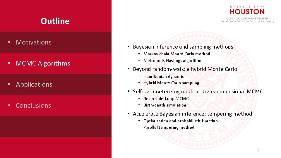
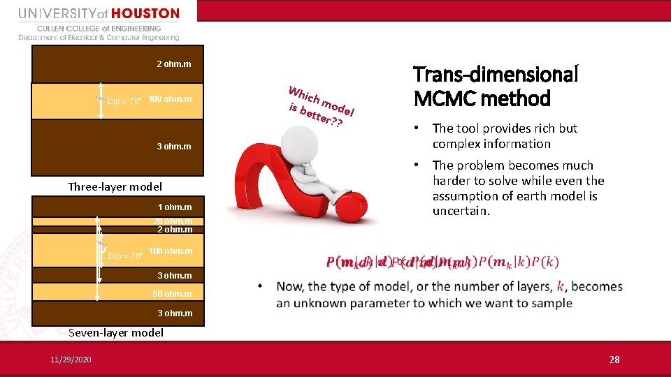
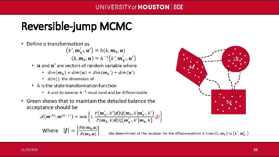
Outline • Motivations • MCMC Algorithms • Applications • Conclusions • Bayesian inference and sampling methods • Markov chain Monte Carlo method • Metropolis-Hastings algorithm • Beyond random-walk: a hybrid Monte Carlo • Hamiltonian dynamic • Hybrid Monte Carlo sampling • Self-parameterizing method: trans-dimensional MCMC • Reversible-jump MCMC • Birth-death simulation • Accelerate Bayesian inference: tempering method • Optimization and probabilistic function • Parallel tempering method 9

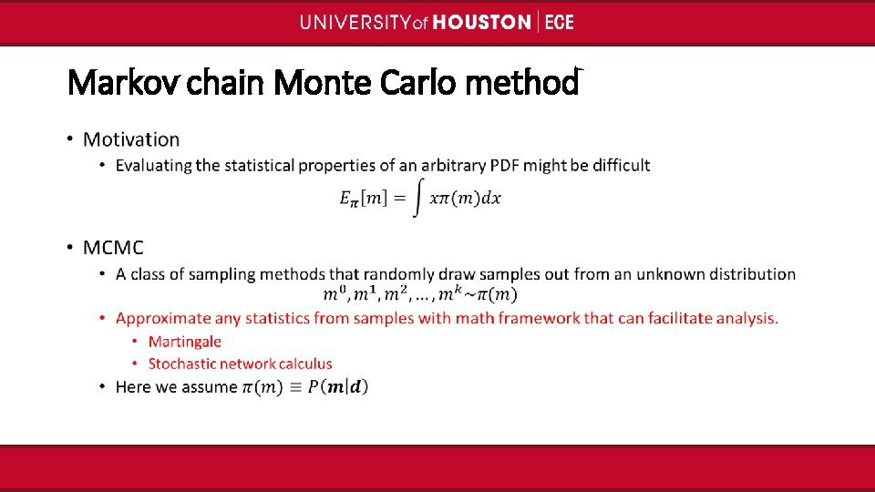
Markov chain Monte Carlo method •

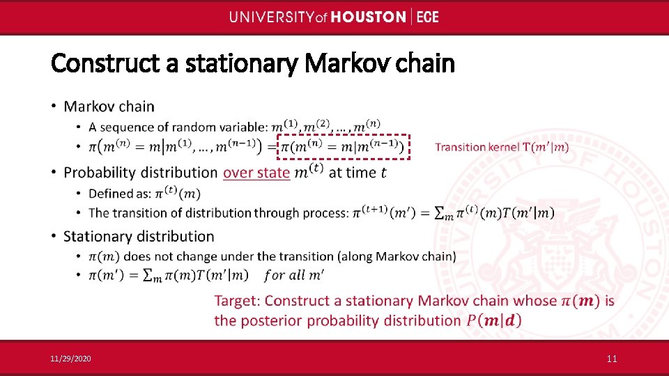
Construct a stationary Markov chain • 11/29/2020 11

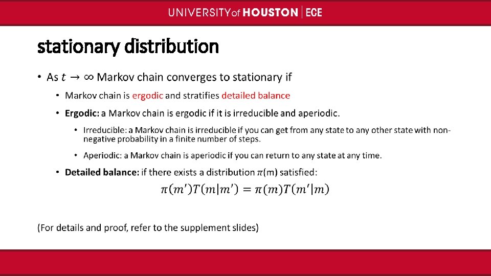
stationary distribution •

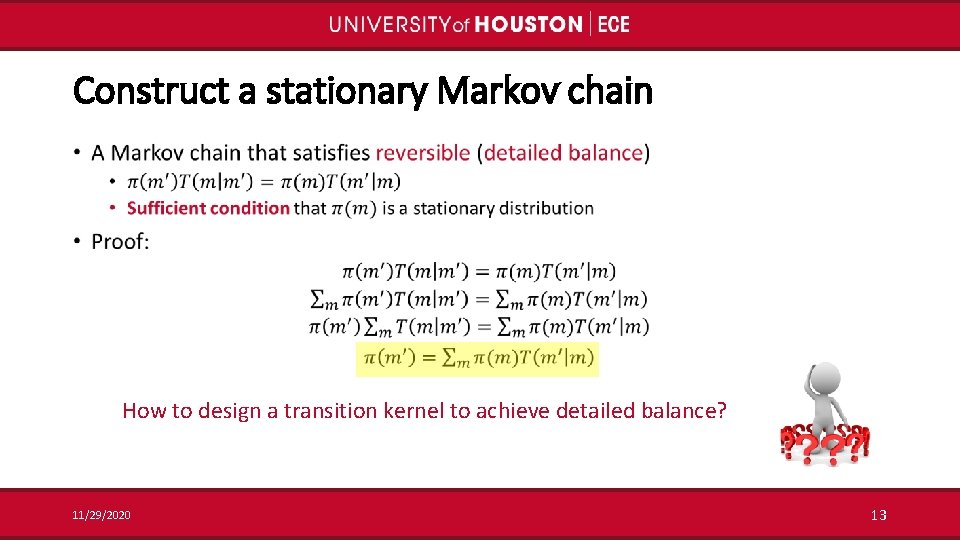
Construct a stationary Markov chain • How to design a transition kernel to achieve detailed balance? 11/29/2020 13

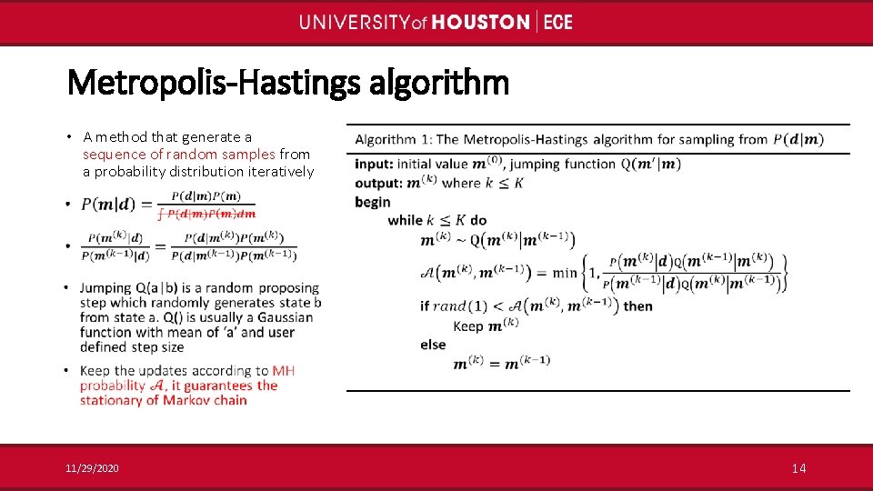
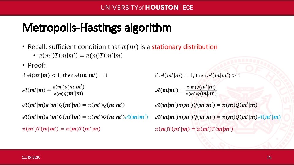
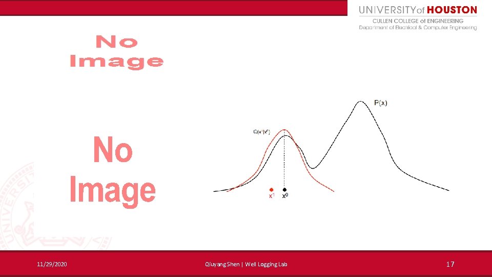
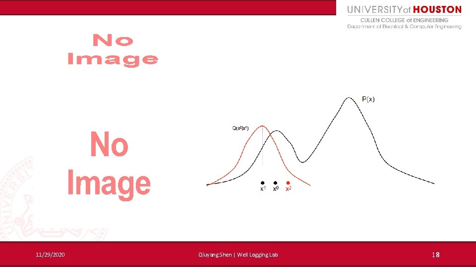
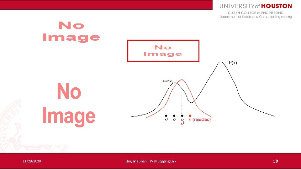
Metropolis-Hastings algorithm • A method that generate a sequence of random samples from a probability distribution iteratively 11/29/2020 14

Metropolis-Hastings algorithm • 11/29/2020 15

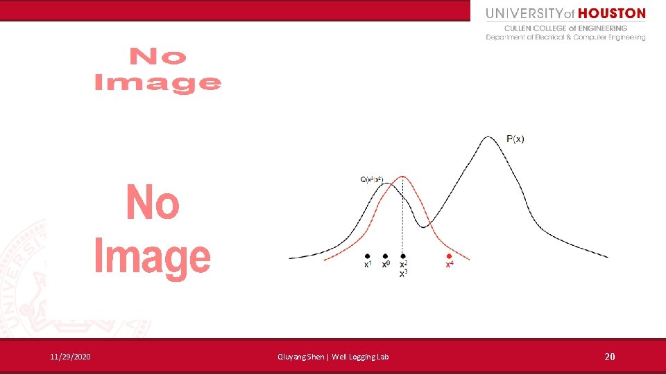
11/29/2020 Qiuyang Shen | Well Logging Lab 16

11/29/2020 Qiuyang Shen | Well Logging Lab 17

11/29/2020 Qiuyang Shen | Well Logging Lab 18

11/29/2020 Qiuyang Shen | Well Logging Lab 19

11/29/2020 Qiuyang Shen | Well Logging Lab 20

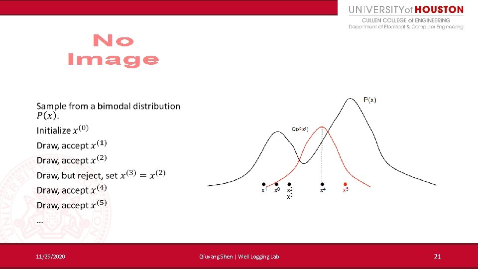
11/29/2020 Qiuyang Shen | Well Logging Lab 21

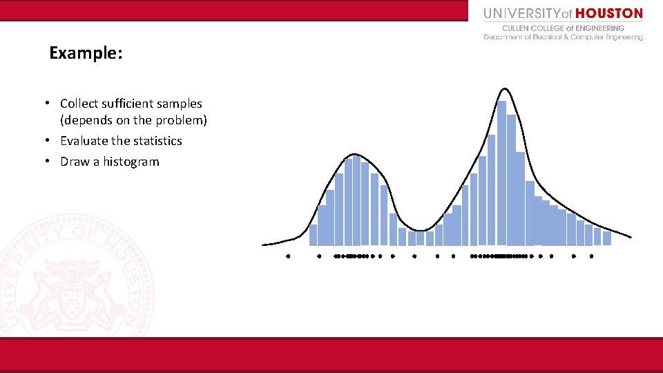
Example: • Collect sufficient samples (depends on the problem) • Evaluate the statistics • Draw a histogram

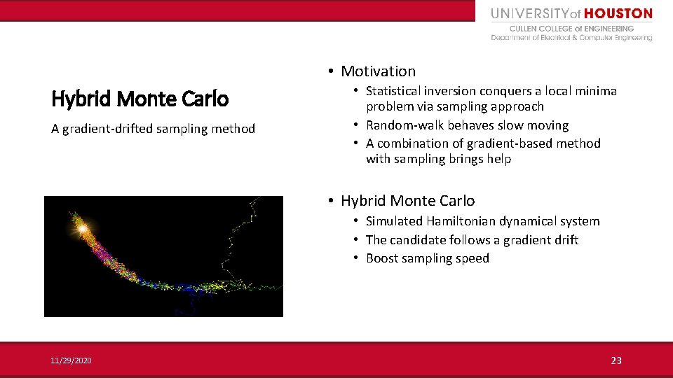
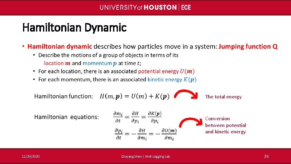
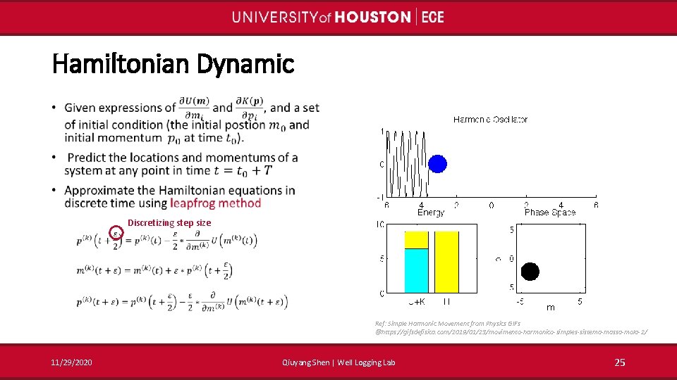
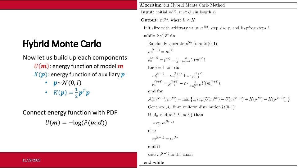
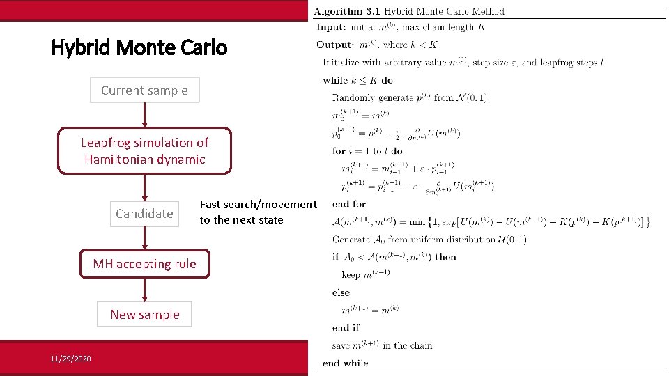
• Motivation Hybrid Monte Carlo A gradient-drifted sampling method • Statistical inversion conquers a local minima problem via sampling approach • Random-walk behaves slow moving • A combination of gradient-based method with sampling brings help • Hybrid Monte Carlo • Simulated Hamiltonian dynamical system • The candidate follows a gradient drift • Boost sampling speed 11/29/2020 23

Hamiltonian Dynamic • The total energy Conversion between potential and kinetic energy 11/29/2020 Qiuyang Shen | Well Logging Lab 24

Hamiltonian Dynamic • Discretizing step size m Ref: Simple Harmonic Movement from Physics GIFs @https: //gifsdefisica. com/2019/01/23/movimento-harmonico-simples-sistema-massa-mola-2/ 11/29/2020 Qiuyang Shen | Well Logging Lab 25

Hybrid Monte Carlo 11/29/2020 26

Hybrid Monte Carlo Current sample Leapfrog simulation of Hamiltonian dynamic Candidate Fast search/movement to the next state MH accepting rule New sample 11/29/2020 27

2 ohm. m Wh ich m od is be tter el ? ? Dip = 78° 100 ohm. m 3 ohm. m 1 ohm. m 20 ohm. m 2 ohm. m 100 ohm. m • The tool provides rich but complex information • The problem becomes much harder to solve while even the assumption of earth model is uncertain. Three-layer model Dip = 78° Trans-dimensional MCMC method 3 ohm. m 50 ohm. m 3 ohm. m Seven-layer model 11/29/2020 28

Reversible-jump MCMC • 2 d 4 d 3 d [1] Green, P. J. and Hastie, D. I. , 2009. Reversible jump MCMC. Genetics, 155(3), pp. 1391 -1403. [2] Green, P. J. , 2003. Trans-dimensional Markov chain monte Carlo. Oxford Statistical Science Series, pp. 179 -198. 11/29/2020 29

Reversible-jump MCMC • 2 d 4 d 3 d 11/29/2020 30

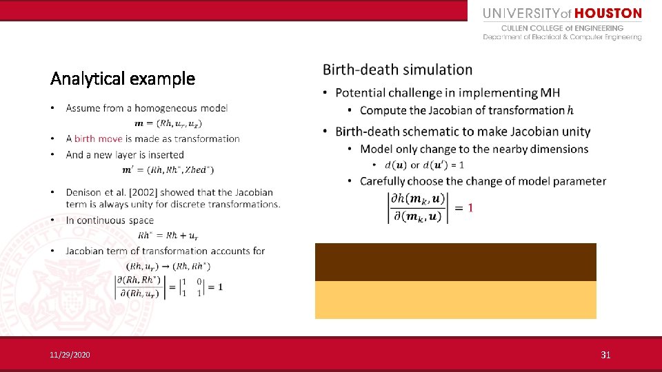
Analytical example • 11/29/2020 31

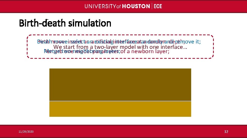
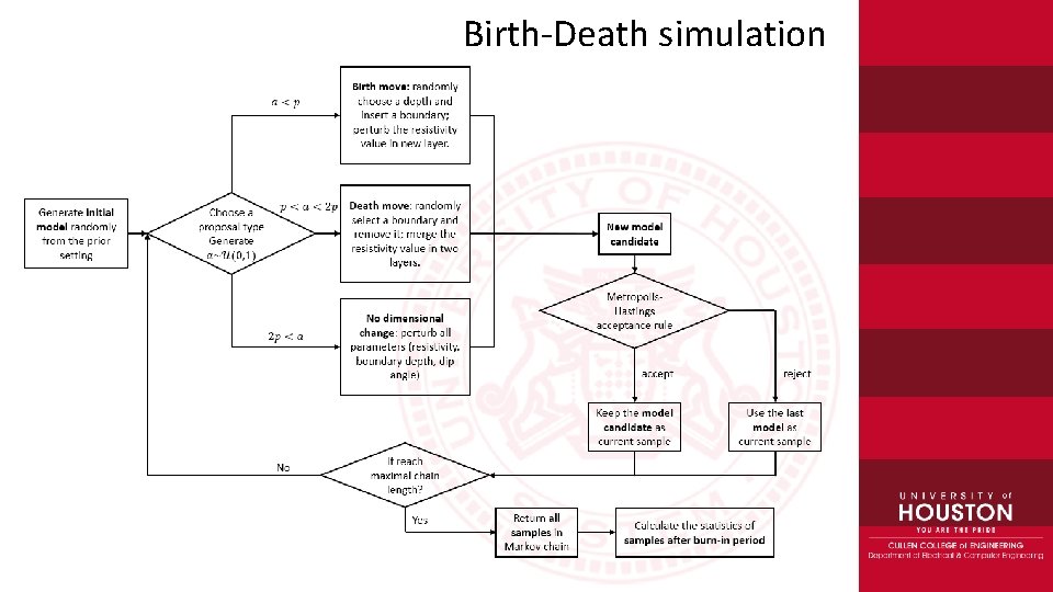
Birth-death simulation Death move: select an existing interface randomly and remove it; Birth move: insert an artificial interface at a random depth; We start from a two-layer model with one interface… Merge two neighboring layers; Perturb one model parameter of a newborn layer; 11/29/2020 32

Birth-Death simulation

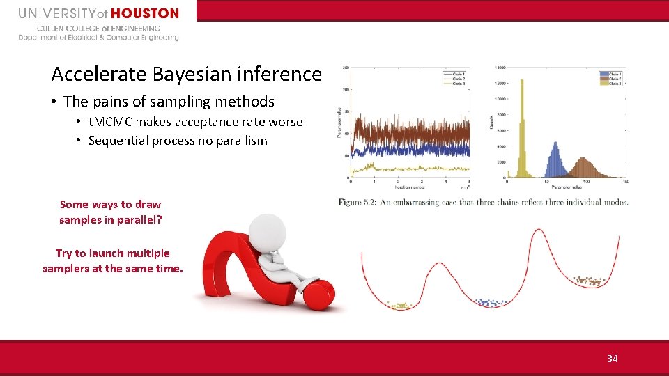
Accelerate Bayesian inference • The pains of sampling methods • t. MCMC makes acceptance rate worse • Sequential process no parallism Some ways to draw samples in parallel? Try to launch multiple samplers at the same time. 34

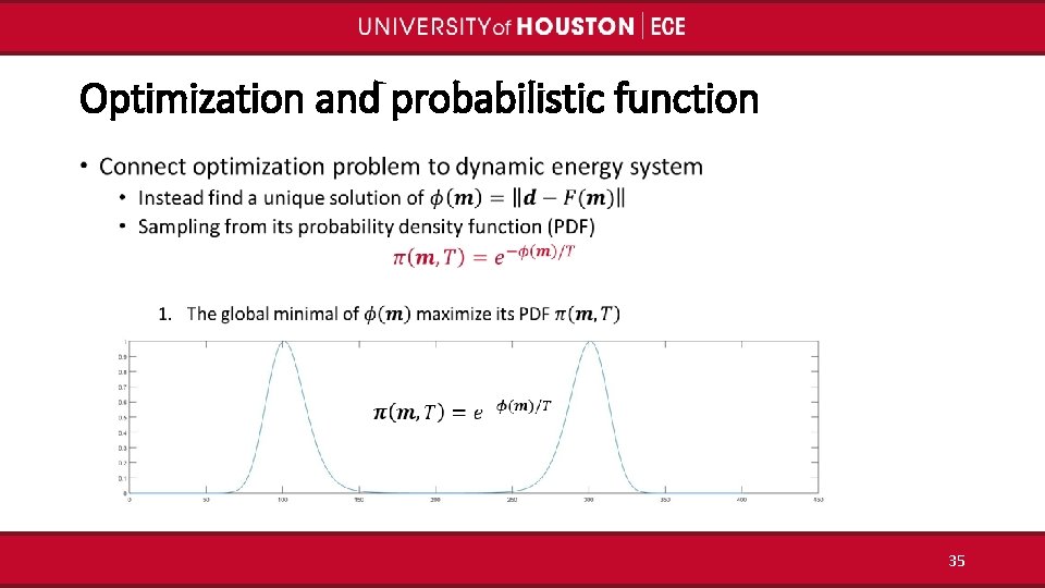
Optimization and probabilistic function • 35

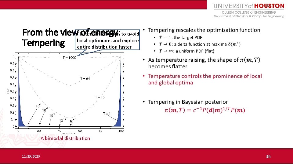
From the view of energy: Flatten distribution to avoid • Tempering local optimums and explore entire distribution faster A bimodal distribution 11/29/2020 36

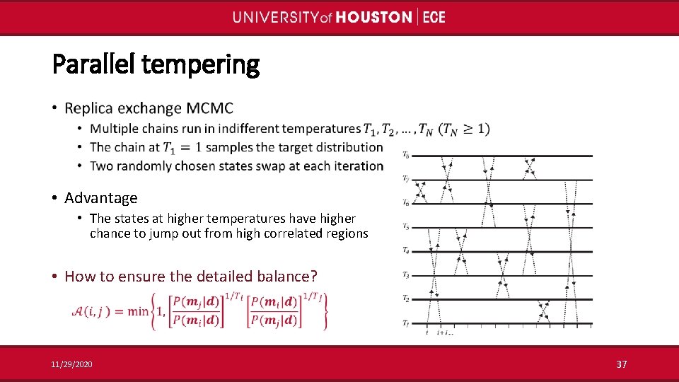
Parallel tempering • • Advantage • The states at higher temperatures have higher chance to jump out from high correlated regions • How to ensure the detailed balance? 11/29/2020 37

Outline • Motivations • MCMC Algorithms • Applications • Conclusions • Oil gas application: earth mode inference using trans-dimensional MCMC algorithm • Communication application: 38

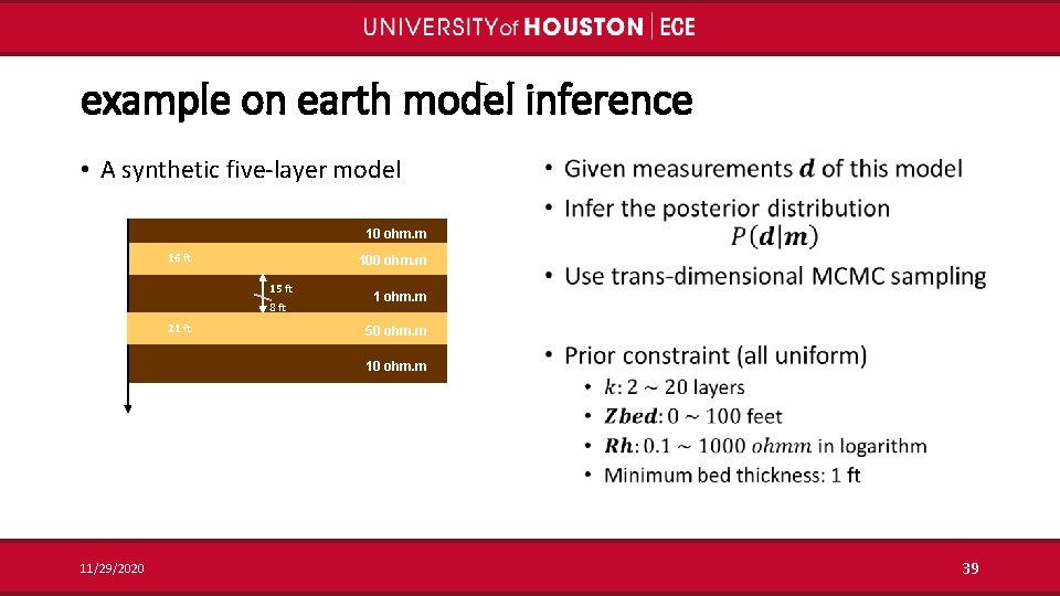
example on earth model inference • A synthetic five-layer model • 10 ohm. m 16 ft 100 ohm. m 15 ft 8 ft 21 ft 1 ohm. m 50 ohm. m 11/29/2020 39

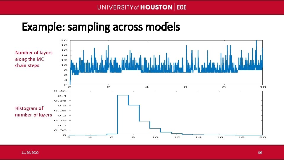
Example: sampling across models Number of layers along the MC chain steps Histogram of number of layers 11/29/2020 40

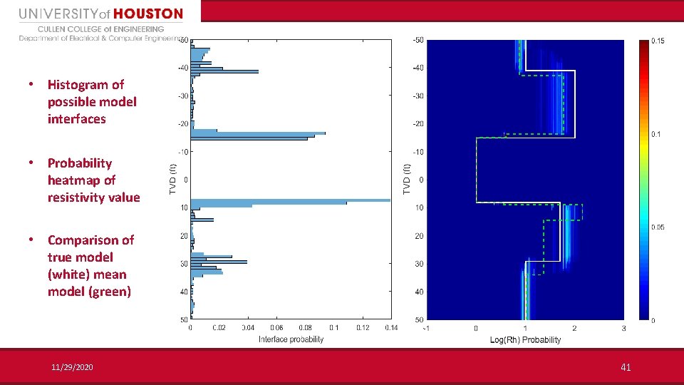
• Histogram of possible model interfaces • Probability heatmap of resistivity value • Comparison of true model (white) mean model (green) 11/29/2020 41

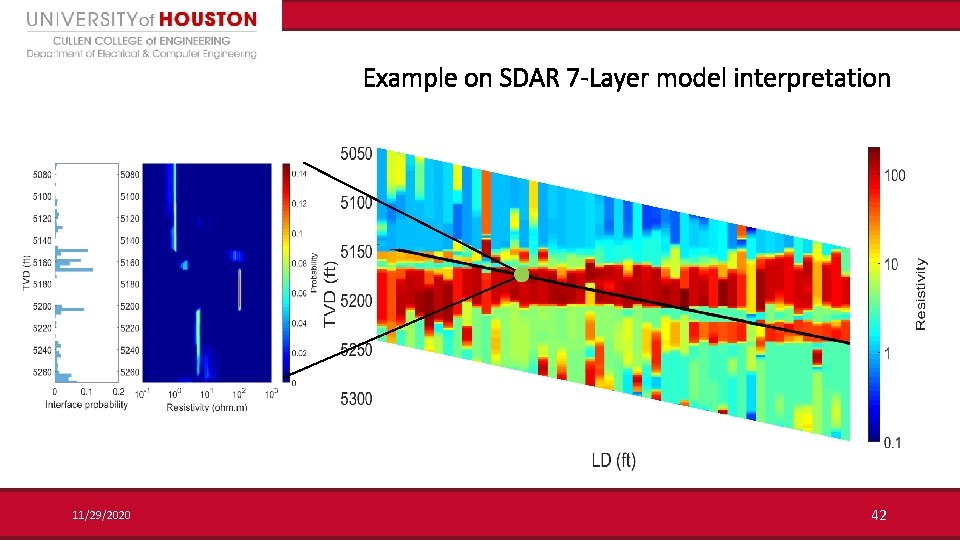
Example on SDAR 7 -Layer model interpretation 11/29/2020 42

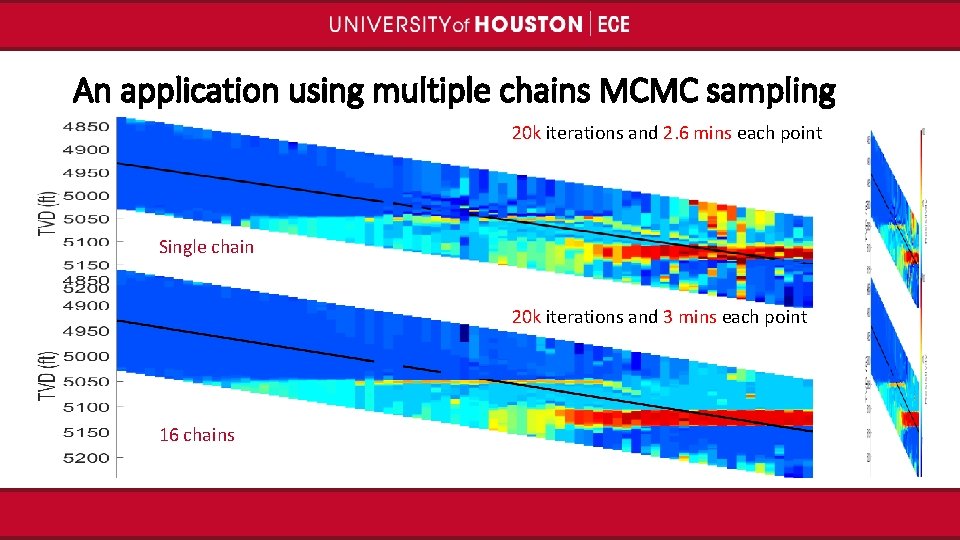
An application using multiple chains MCMC sampling 20 k iterations and 2. 6 mins each point Single chain 20 k iterations and 3 mins each point 16 chains

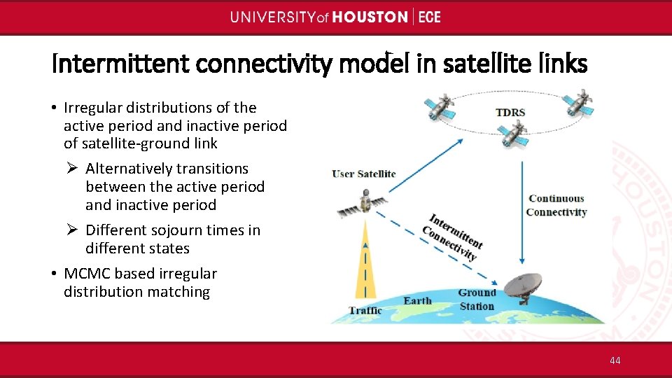
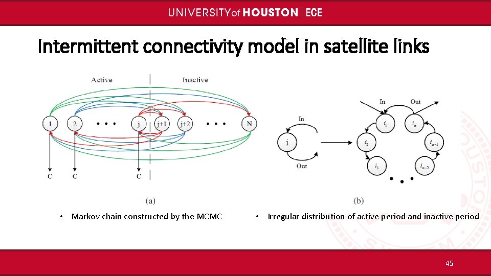
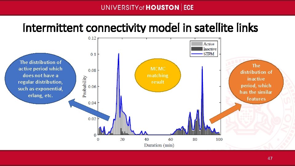
Intermittent connectivity model in satellite links • Irregular distributions of the active period and inactive period of satellite-ground link Ø Alternatively transitions between the active period and inactive period Ø Different sojourn times in different states • MCMC based irregular distribution matching 44

Intermittent connectivity model in satellite links • Markov chain constructed by the MCMC • Irregular distribution of active period and inactive period 45

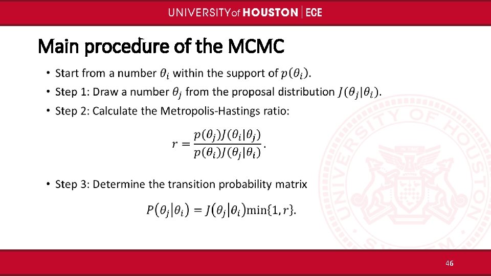
Main procedure of the MCMC 46

Intermittent connectivity model in satellite links The distribution of active period which does not have a regular distribution, such as exponential, erlang, etc. MCMC matching result The distribution of inactive period, which has the similar features 47

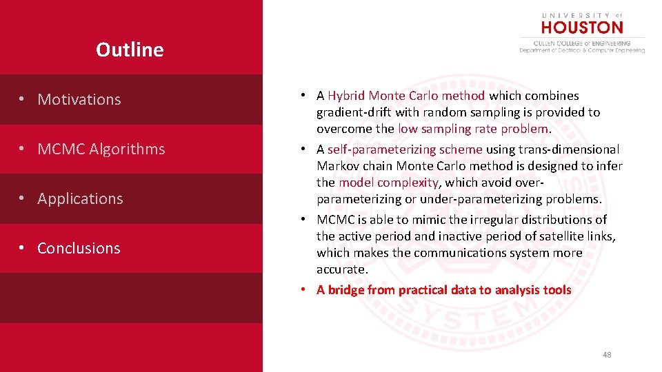
Outline • Motivations • MCMC Algorithms • Applications • Conclusions • A Hybrid Monte Carlo method which combines gradient-drift with random sampling is provided to overcome the low sampling rate problem. • A self-parameterizing scheme using trans-dimensional Markov chain Monte Carlo method is designed to infer the model complexity, which avoid overparameterizing or under-parameterizing problems. • MCMC is able to mimic the irregular distributions of the active period and inactive period of satellite links, which makes the communications system more accurate. • A bridge from practical data to analysis tools 48

Q&A “Iron and Thunder” by Patrick Soper

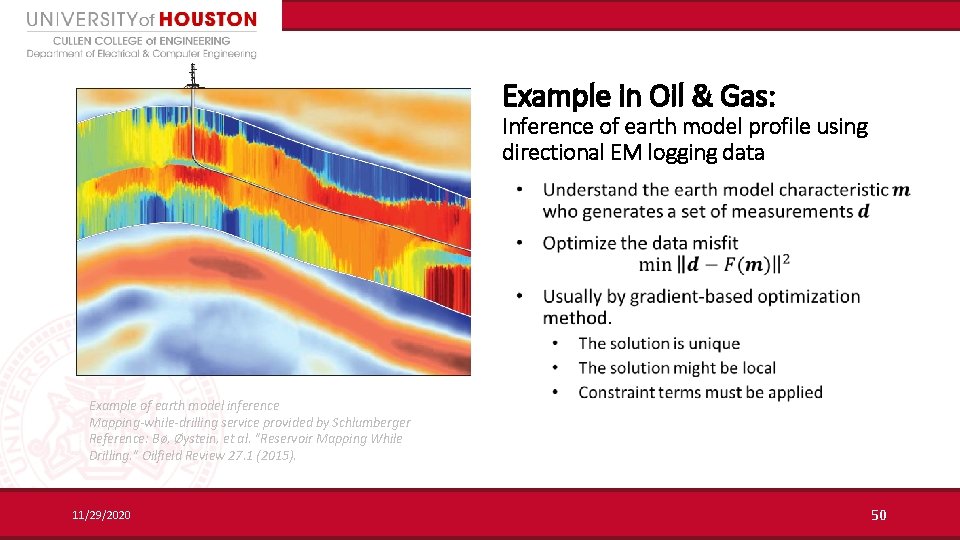
Example in Oil & Gas: Inference of earth model profile using directional EM logging data Example of earth model inference Mapping-while-drilling service provided by Schlumberger Reference: Bø, Øystein, et al. "Reservoir Mapping While Drilling. " Oilfield Review 27. 1 (2015). 11/29/2020 50

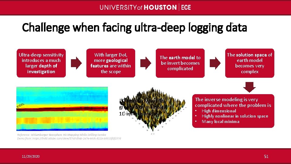
Challenge when facing ultra-deep logging data Ultra-deep sensitivity introduces a much larger depth of investigation With larger Do. I, more geological features are within the scope The earth model to be invert becomes complicated 2 D resistivity profile grouped by multiple 1 D inverse results The solution space of earth model becomes very complex The inverse modeling is very complicated where the problem is • • • High dimensional Highly nonlinear in solution space Many local minima Reference: Schlumberger Geosphere HD Mapping While Drilling Service Demo from: https: //indd. adobe. com/view/37 a 5 d 5 eb-2 e 7 e-44 dc-811 b-b 0 d 23 f 0 f 257 d 11/29/2020 51