Tutorial Calibrated Rectification Using Open CV Bouguets Algorithm

Tutorial: Calibrated Rectification Using Open. CV (Bouguet’s Algorithm) Michael Hornáček Stereo Vision VU 2013 Vienna University of Technology

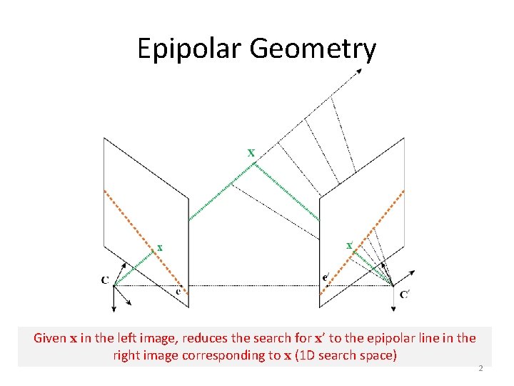
Epipolar Geometry Given x in the left image, reduces the search for x’ to the epipolar line in the right image corresponding to x (1 D search space) 2

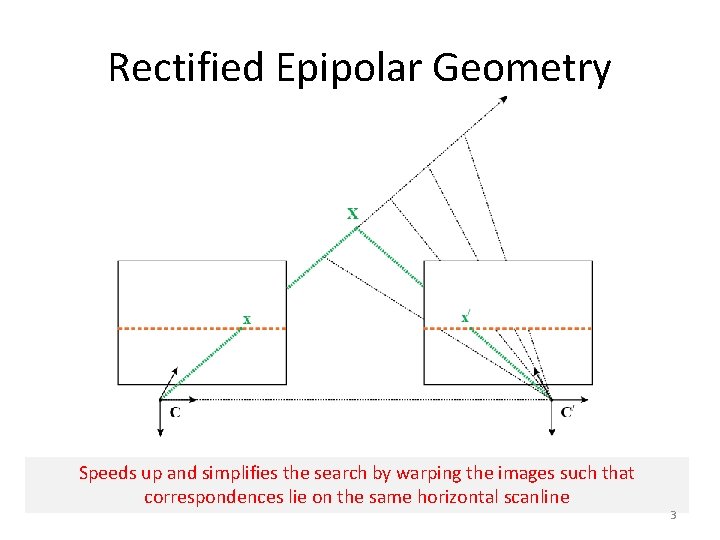
Rectified Epipolar Geometry Speeds up and simplifies the search by warping the images such that correspondences lie on the same horizontal scanline 3

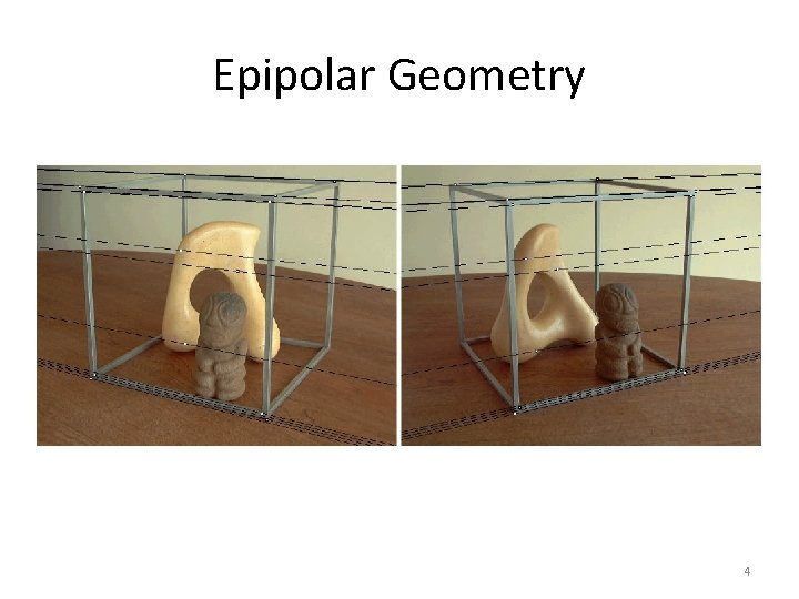
Epipolar Geometry 4

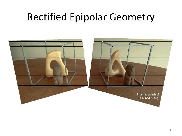
Rectified Epipolar Geometry From approach of Loop and Zhang 5

Homogeneous Coordinates

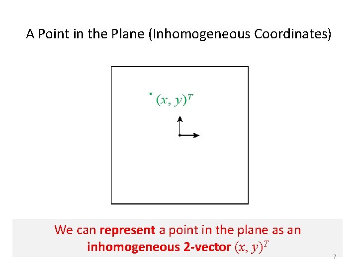
A Point in the Plane (Inhomogeneous Coordinates) We can represent a point in the plane as an inhomogeneous 2 -vector (x, y)T 7

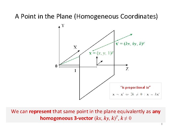
A Point in the Plane (Homogeneous Coordinates) “is proportional to” We can represent that same point in the plane equivalently as any homogeneous 3 -vector (kx, ky, k)T, k ≠ 0 8

Homogeneous vs. Inhomogeneous The homogeneous 3 -vector x ~ (kx, ky, k)T represents the same point in the plane as the inhomogenous 2 -vector x^ = (kx/k, ky/k)T = (x, y)T Generalizes to higher-dimensional spaces 9

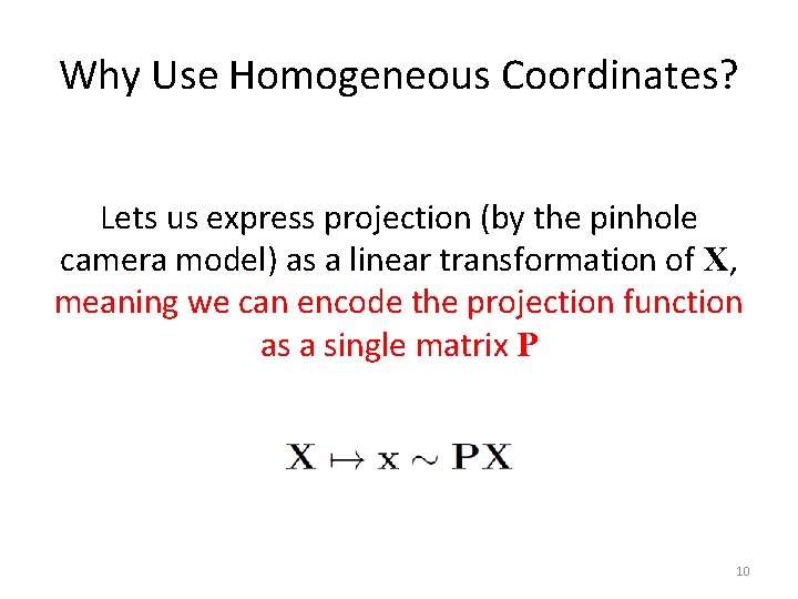
Why Use Homogeneous Coordinates? Lets us express projection (by the pinhole camera model) as a linear transformation of X, meaning we can encode the projection function as a single matrix P 10

Pinhole Camera Model

(xcam, ycam)T: Projected Pt in Camera Coordinates [mm] ^ Canonical pose: camera center C is at origin 0 of world coordinate frame, camera is facing in positive Z-direction with xcam and ycam aligned with the Xand Y-axes, respectively 12

(xcam, ycam)T: Projected Pt in Camera Coordinates [mm] 13

(xcam, ycam)T: Projected Pt in Camera Coordinates [mm] 14

(xcam, ycam)T: Projected Pt in Camera Coordinates [mm] 15

(xcam, ycam)T: Projected Pt in Camera Coordinates [mm] 16

(xcam, ycam)T: Projected Pt in Camera Coordinates [mm] 17

(xcam, ycam)T: Projected Pt in Camera Coordinates [mm] 18

(xim, yim)T: Projected Pt in Image Coordinates [mm] 19

(xim, yim)T: Projected Pt in Image Coordinates [mm] w/2 0 w/2 w 0 common assumption px = w / 2 py = h / 2 h/2 h 20

(xpx, ypx)T: Projected Pt in Pixel Coordinates [px] mx = wpx [px] w [mm] hpx [px] my = h [mm] xim = f. X/Z+px [mm] yim = f. Y/Z+py [mm] 21

(xpx, ypx)T: Projected Pt in Pixel Coordinates [px] invertible 3 x 3 camera calibration matrix K 22

Omitted for Brevity: Distortions and Skew Typically pixel skew is disregarded and images can be undistorted in a pre-processing step using distortion coefficients obtained during calibration, allowing us to use the projection matrix presented 23

Pinhole Camera in Noncanonical Pose

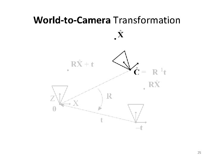
World-to-Camera Transformation 25

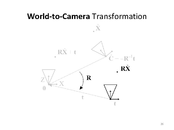
World-to-Camera Transformation 26

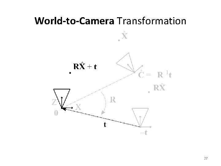
World-to-Camera Transformation 27

World-to-Camera Transformation ^ We now project ((RX + t)T, 1)T using [K | 0] as before 28

(xpx, ypx)T: Projected Pt in Pixel Coordinates [px] for Camera in Non-canonical Pose invertible 4 x 4 world-to-camera rigid body transformation matrix We use this decomposition rather than the equivalent and more common P = K[R | t] since it will allow us to reason more easily about combinations of rigid body transformation matrices 29

Geometry of Two Views

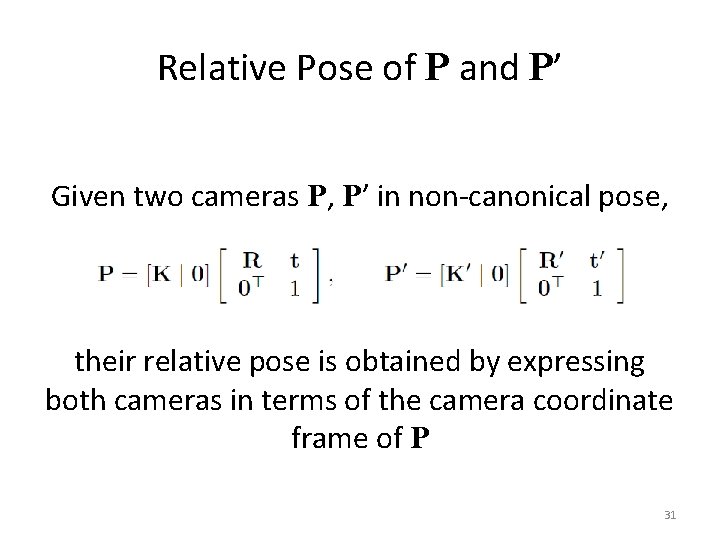
Relative Pose of P and P’ Given two cameras P, P’ in non-canonical pose, their relative pose is obtained by expressing both cameras in terms of the camera coordinate frame of P 31

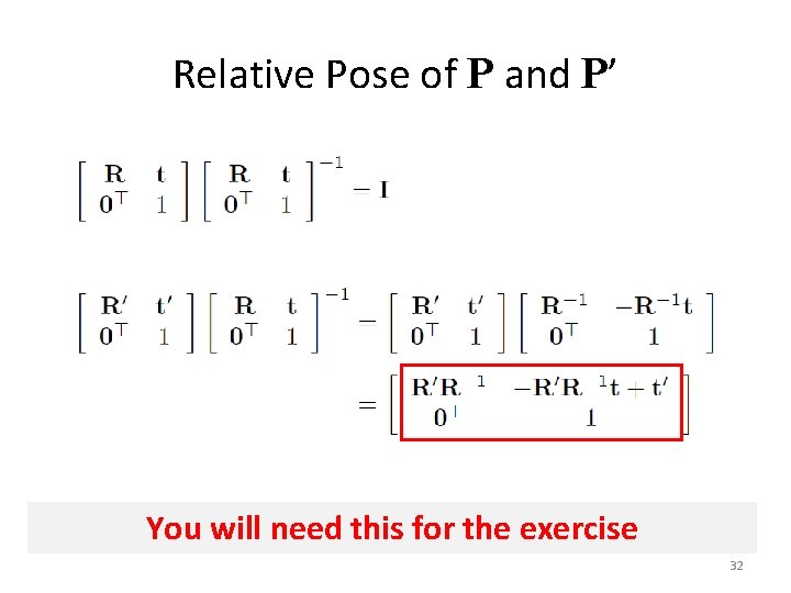
Relative Pose of P and P’ You will need this for the exercise 32

Rotation about the Camera Center

Rotation about the Camera Center Rectifying our cameras will involve rotating them about their respective camera center, from which we obtain the corresponding pixel transformations for warping the images 34

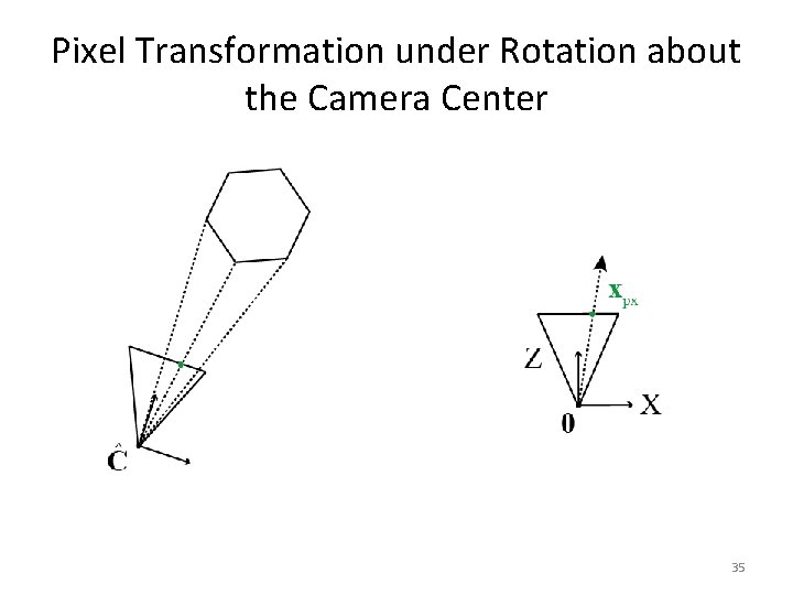
Pixel Transformation under Rotation about the Camera Center 35

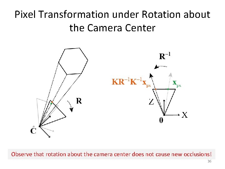
Pixel Transformation under Rotation about the Camera Center Observe that rotation about the camera center does not cause new occlusions! 36

Rectification via Bouguet’s Algorithm (Sketch)

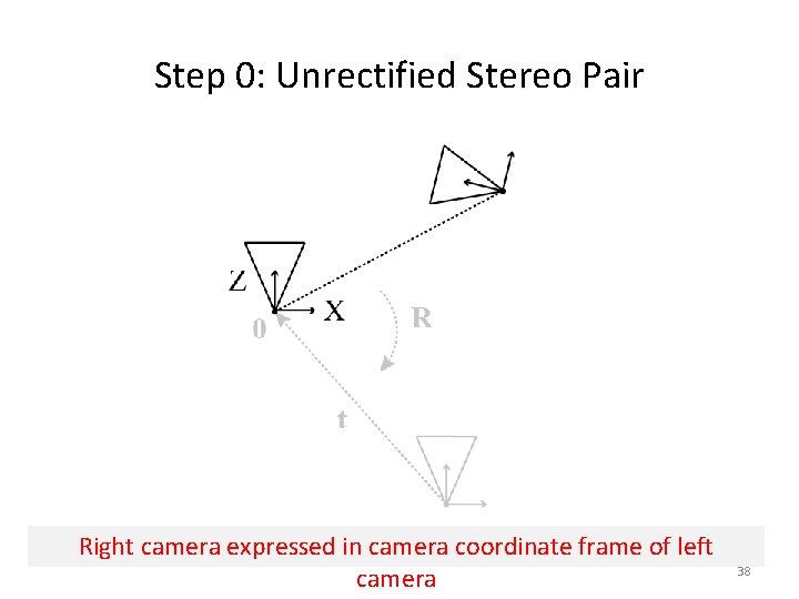
Step 0: Unrectified Stereo Pair Right camera expressed in camera coordinate frame of left camera 38

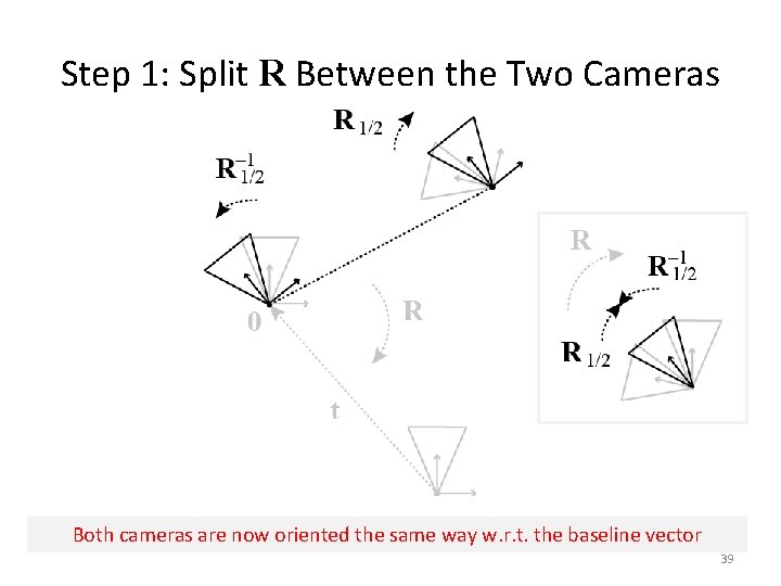
Step 1: Split R Between the Two Cameras Both cameras are now oriented the same way w. r. t. the baseline vector 39

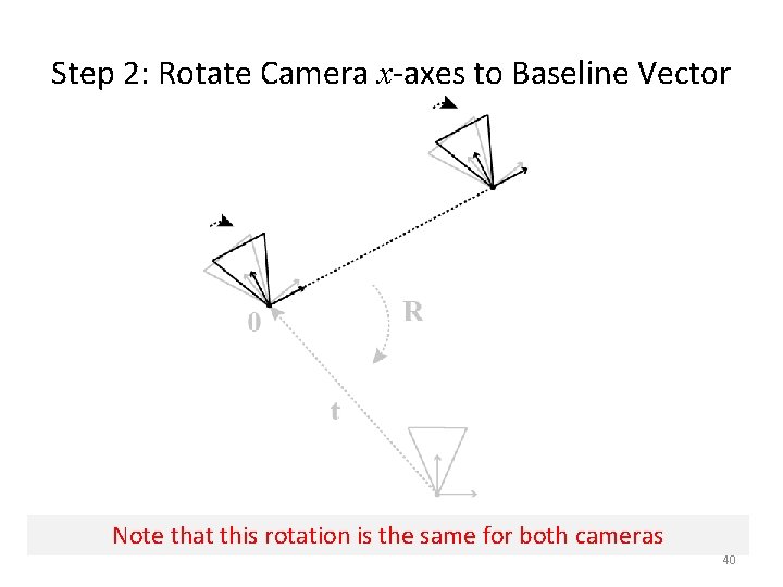
Step 2: Rotate Camera x-axes to Baseline Vector Note that this rotation is the same for both cameras 40

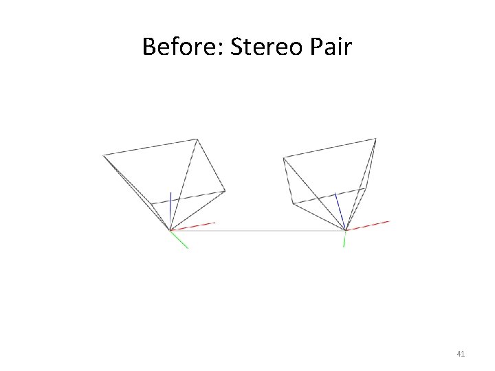
Before: Stereo Pair 41

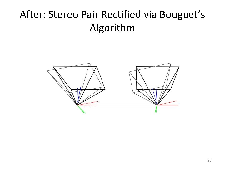
After: Stereo Pair Rectified via Bouguet’s Algorithm 42

Bouguet’s Algorithm in Open. CV

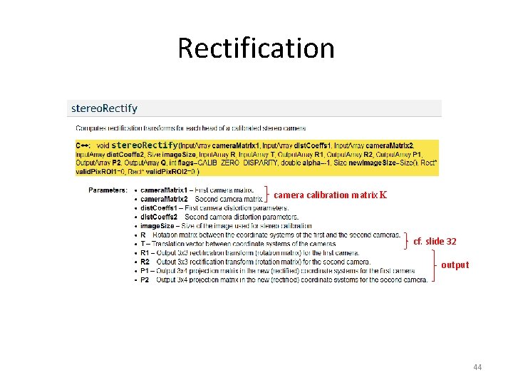
Rectification camera calibration matrix K cf. slide 32 output 44

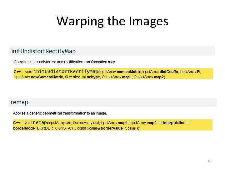
Warping the Images 45

Literature G. Bradsky and A. Kaehler, Learning Open. CV: Computer Vision with the Open. CV Library, 2004, O’Reilly, Sebastopol, CA. S. Birchfield. “An Introduction to Projective Geometry (for computer vision), ” 1998, http: //robotics. stanford. edu/~birch/projective/. R. Hartley and A. Zisserman, Multiple View Geometry in Computer Vision, 2004, Cambridge University Press, Cambridge, UK. Y. Ma et al. , An Invitation to 3 -D Vision, 2004, Springer Verlag, New York, NY. C. Loop and Z. Zhang, “Computing Rectifying Homographies for Stereo Vision, ” in CVPR, 1999. 46

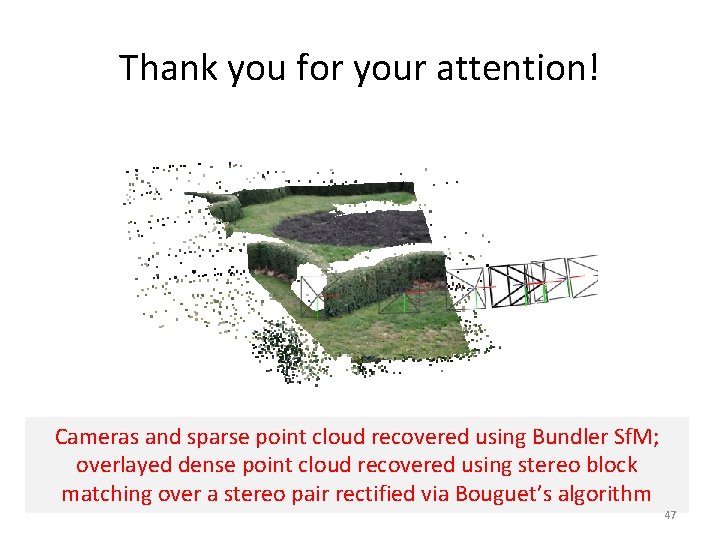
Thank you for your attention! Cameras and sparse point cloud recovered using Bundler Sf. M; overlayed dense point cloud recovered using stereo block matching over a stereo pair rectified via Bouguet’s algorithm 47