Tutorial 3 spectral functions for SIAM arbitrary DOS

Tutorial 3: spectral functions for SIAM, arbitrary DOS, finite-tempratures, T-matrix for Kondo model Rok Žitko Institute Jožef Stefan Ljubljana, Slovenia
![Spectral funcion 05_spec [param] symtype=QS discretization=C Lambda=2 Tmin=1 e-10 keepenergy=10 keep=5000 model=SIAM U=0. 01](http://slidetodoc.com/presentation_image_h2/b1ddc04ce195029245ffe632ea468ef8/image-2.jpg "Spectral funcion 05_spec [param] symtype=QS discretization=C Lambda=2 Tmin=1 e-10 keepenergy=10 keep=5000 model=SIAM U=0. 01")
Spectral funcion 05_spec [param] symtype=QS discretization=C Lambda=2 Tmin=1 e-10 keepenergy=10 keep=5000 model=SIAM U=0. 01 Gamma=0. 001 delta=0 ops=A_d specd=A_d-A_d creation/annihilation operator spectral function <<d; d†>> broaden_max=0. 1 broaden_min=1 e-7 broaden_ratio=1. 02 fdm=true T=1 e-10 smooth=new alpha=0. 6 omega 0=1 e-99 grid for the broadened (smooth) spectral function full-density-matrix method temperature for the spectral-function calculation broadening parameters

Output: spectral function = imaginary part of the Green's function The corresponding real part can be computed using the Kramers-Kronig transformation tool "kk", which comes bundled as part of the NRG Ljubljana package.

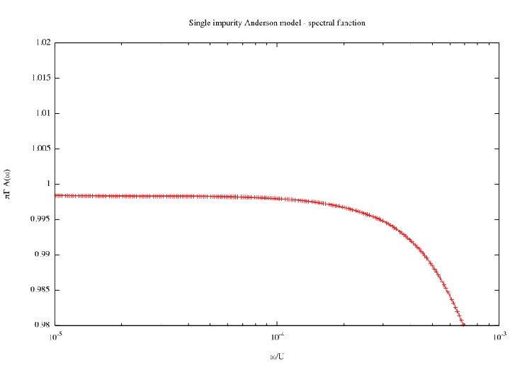
2 a_plot

2 a_plot_log

2 a_plot_log_friedel
![Removing oscillations using the z-averaging #!/usr/bin/env looper #AUTOLOOP: nrginit ; nrgrun #OVERWRITE [param] symtype=QS](http://slidetodoc.com/presentation_image_h2/b1ddc04ce195029245ffe632ea468ef8/image-7.jpg "Removing oscillations using the z-averaging #!/usr/bin/env looper #AUTOLOOP: nrginit ; nrgrun #OVERWRITE [param] symtype=QS")
Removing oscillations using the z-averaging #!/usr/bin/env looper #AUTOLOOP: nrginit ; nrgrun #OVERWRITE [param] symtype=QS discretization=Z @$z = 1/4; $z <= 1; $z += 1/4 z=$z Lambda=2 Tmin=1 e-10 keepenergy=10 keep=10000 model=SIAM U=0. 01 Gamma=0. 001 delta=0 ops=A_d specd=A_d-A_d broaden_max=0. 1 broaden_min=1 e-8 broaden_ratio=1. 02 fdm=true T=1 e-10 smooth=new alpha=0. 3 omega 0=1 e-99 May be reduced! 05_spec_z/1_zloop

05_spec_z/2_proc #!/bin/sh FN=spec_FDM_dens_A_d-A_d. dat Nz=4 intavg ${FN} ${Nz} Gamma=`getparam Gamma 1_zloop` U=`getparam U 1_zloop` scaley=`echo 3. 14159*${Gamma} | bc` scalex=`echo 1/${U} | bc` scalexy ${scalex} ${scaley} ${FN} >A-rescaled. dat intavg is a tool for z-averaging the spectral functions

Exercises 1. Try increasing L. How do the results deteriorate? 2 a 1 2. Try changing the broadening a and the number of z points. When do the oscillations appear? 3. How does the Kondo resonance evolve as U is decreased toward 0?
 trick")
Self-energy (S) trick

12_self_energy_trick/1_zloop #!/usr/bin/env looper #PRELUDE: $Nz=8; #AUTOLOOP: nrginit ; nrgrun #OVERWRITE model=. . /model. m U=0. 5 Gamma=0. 03 delta=0. 1 [sweep] Nz=8 ops=A_d self_d specd=A_d-A_d self_d-A_d [param] symtype=QS Lambda=2. 0 Tmin=1 e-8 keepmin=200 keepenergy=10. 0 keep=10000 dmnrg=true good. E=2. 3 NN 2 avg=true discretization=Z @$z = 1/$Nz; $z <= 1. 00001; $z += 1/$Nz z=$z # Broadening is performed by an external tool broaden_max=2 broaden_ratio=1. 01 broaden_min=1 e-6 bins=1000 broaden=false savebins=true T=1 e-10
![12_self_energy_trick/model. m def 1 ch[1]; H = H 0 + Hc + H 1;](http://slidetodoc.com/presentation_image_h2/b1ddc04ce195029245ffe632ea468ef8/image-13.jpg "12_self_energy_trick/model. m def 1 ch[1]; H = H 0 + Hc + H 1;")
12_self_energy_trick/model. m def 1 ch[1]; H = H 0 + Hc + H 1; (* All operators which contain d[], except hybridization (Hc). *) Hselfd = H 1; selfopd = ( Chop @ Expand @ komutator[Hselfd /. params, d[#1, #2]] )&; (* Evaluate *) Print["selfopd[CR, UP]=", Print["selfopd[CR, DO]=", Print["selfopd[AN, UP]=", Print["selfopd[AN, DO]=", selfopd[CR, selfopd[AN, UP]]; DO]]; H 0 = Hamiltonian for the first site (index 0) of the Wilson chain Hc = hybridization part of the Hamiltonian, hopping between the impurity and the first site of the Wilson chain H 1 = the impurity Hamiltonian
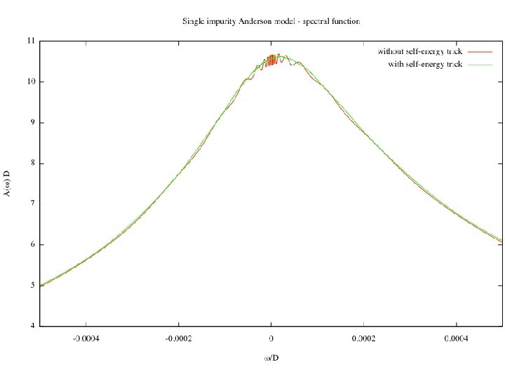
 and AF (self_d-A_d) • compute")
Postprocessing • z-averaging of both spectral functions, AG (A_d-A_d) and AF (self_d-A_d) • compute the corresponding real parts to obtain the full Green's functions: G=Re G-ip AG, similarly for F • compute the self-energy • calculate the improved spectral function average realparts sigmatrick

3 a_plot

3 b_plot_zoom

3 c_plot_F

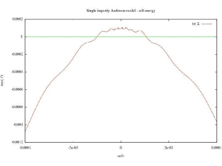
3 d_plot_sigma

3 e_plot_sigma_zoom Re S - linear Im S - quadratic

Exercises 1. Extract the quasiparticle renormalization factor Z, defined as How does it vary with U? Is it related to TK? 2. Is Im S really quadratic? Is its curvature related to Z?

FDM, L=4, Nz=2, a=0. 5

Arbitrary density of states pseudogap 13_arbitrary_DOS
![02_zloop [param] symtype=QS Lambda=2. 0 Tmin=1 e-8 keepmin=200 keepenergy=10. 0 keep=10000 band=asymode dos=. .](http://slidetodoc.com/presentation_image_h2/b1ddc04ce195029245ffe632ea468ef8/image-25.jpg "02_zloop [param] symtype=QS Lambda=2. 0 Tmin=1 e-8 keepmin=200 keepenergy=10. 0 keep=10000 band=asymode dos=. .")
02_zloop [param] symtype=QS Lambda=2. 0 Tmin=1 e-8 keepmin=200 keepenergy=10. 0 keep=10000 band=asymode dos=. . /Delta. dat discretization=Z @$z = 1/$Nz; $z <= 1. 00001; $z += 1/$Nz z=$z param [param] xmax=20 dos=Delta. dat for "adapt" tool which solves the discretization ODE
 for positive")
Diagonalization tool "adapt" Input: Delta. dat Output: FSOL. dat, FSOLNEG. dat f(x) for positive and negative frequencies Invocation: adapt P adapt N

4 c_plot_FSOL

4 a_plot

4 b_plot_zoom

4 e_plot_sigma

4 f_plot_sigma_zoom

Exercises • Try some other densities of states in the band. How robust is the Kondo resonance? • When d=0, show that the model is not particle -hole symmetric if the band isn't. • Can the code handle discontinuities in DOS? What about divergencies in DOS?

Finite-temperature spectral functions 05_spec_ft/1 e-3 ops=A_d specd=A_d-A_d broaden_max=0. 1 broaden_min=1 e-7 broaden_ratio=1. 02 fdm=true T=1 e-3 Full density matrix method (recommended for finite T) smooth=new alpha=0. 6 Broadening kernel for finite T

1 a_plot

1 b_plot_zoom

Exercises • Combine the code for the self-energy trick with that for finite-T calculations (using FDM NRG). How does Im S evolve with increasing temperature?

Kondo model
![#!/usr/bin/env looper #AUTOLOOP: nrginit ; nrgrun #OVERWRITE [extra] spin=1/2 Jkondo=0. 2 [param] symtype=QS discretization=Z](http://slidetodoc.com/presentation_image_h2/b1ddc04ce195029245ffe632ea468ef8/image-38.jpg "#!/usr/bin/env looper #AUTOLOOP: nrginit ; nrgrun #OVERWRITE [extra] spin=1/2 Jkondo=0. 2 [param] symtype=QS discretization=Z")
#!/usr/bin/env looper #AUTOLOOP: nrginit ; nrgrun #OVERWRITE [extra] spin=1/2 Jkondo=0. 2 [param] symtype=QS discretization=Z @$z = 1/4; $z <= 1; $z += 1/4 z=$z Lambda=2 Tmin=1 e-10 keepenergy=10 keep=10000 model=. . /kondo. m ops=hyb_f Sf. Sk specd=hyb_f-hyb_f broaden_max=0. 1 broaden_min=1 e-8 broaden_ratio=1. 02 fdm=true T=1 e-11 smooth=new alpha=0. 3 omega 0=1 e-99 05_spec_kondo/1_zloop
![def 1 ch[0]; 05_spec_kondo/model. m SPIN = To. Expression @ param["spin", "extra"]; Module[{sx, sy,](http://slidetodoc.com/presentation_image_h2/b1ddc04ce195029245ffe632ea468ef8/image-39.jpg "def 1 ch[0]; 05_spec_kondo/model. m SPIN = To. Expression @ param[\"spin\", \"extra\"]; Module[{sx, sy,")
def 1 ch[0]; 05_spec_kondo/model. m SPIN = To. Expression @ param["spin", "extra"]; Module[{sx, sy, sz, ox, oy, oz, ss}, sx = spinketbra. X[SPIN]; sy = spinketbra. Y[SPIN]; sz = spinketbra. Z[SPIN]; ox = nc[ sx, spinx[ f[0] ] ]; oy = nc[ sy, spiny[ f[0] ] ]; oz = nc[ sz, spinz[ f[0] ] ]; ss = Expand[ox + oy + oz]; Hk = Jkondo ss; ]; H = H 0 + Hk; Hhyb = Hk; MAKESPINKET = SPIN; hybopf = ( Chop @ Expand @ komutator[Hhyb /. params, f[#1, 0, #2]] )&; NOTE: this is different from what we did in SIAM for the self-energy trick, where we computed the commutator with the interaction part of the Hamiltonian.
![Module[{t={}}, If[calcopq["hyb_f"], Append. To[t, {"dhyb_f"}]; MPVCFAST = False; t = Join[t, ireduc. Table[ hybopf](http://slidetodoc.com/presentation_image_h2/b1ddc04ce195029245ffe632ea468ef8/image-40.jpg "Module[{t={}}, If[calcopq[\"hyb_f\"], Append. To[t, {\"dhyb_f\"}]; MPVCFAST = False; t = Join[t, ireduc. Table[ hybopf")
Module[{t={}}, If[calcopq["hyb_f"], Append. To[t, {"dhyb_f"}]; MPVCFAST = False; t = Join[t, ireduc. Table[ hybopf ]]; MPVCFAST = True; ]; texportable = t; ]; texportable 05_spec_kondo/modeloperators. m

3 a_plot

3 b_plot_zoom
 of the Kondo resonance related to the")
Exercises • How is the width (HWHM) of the Kondo resonance related to the Kondo temperature TK?
- Slides: 43