Tutorial 2 SEG 7550 Introduction to MATLAB II

Tutorial 2 SEG 7550 Introduction to MATLAB II 25 th, Sep. , 2009

Outline l Source of financial data l Generate graphs in MATLAB l Review programs in class

Histogram plot l n = hist(Y) bins the elements in vector Y into 10 equally spaced containers and returns the number of elements in each container as a row vector. l n = hist(Y, x) where x is a vector, returns the distribution of Y among length(x) bins with centers specified by x. For example, if x is a 5 -element vector, hist distributes the elements of Y into five bins centered on the x-axis at the elements in x, none of which can be complex.

Histogram plot l Example: x = -4: 0. 1: 4; y = randn(10000, 1); hist(y, x)

Plot (basic) l plot(X, Y) plots vector Y versus vector X. l plot(Y) plots the columns of Y versus their index l Title: use function ‘title()’ l X, Y axis labels: use function ‘xlabel()’ and ‘ylabel() ’

Plot multiple data sets in one graph l Example: X=0: 0. 1: 10; Y 1=X. ^2 -10. *X+15; Y 2=-X. ^2+10. *X; Y 3=0. 5. *(X. ^2); plot(X, Y 1, X, Y 3) title(‘graph’) xlabel(‘x’) ylabel(‘y’)

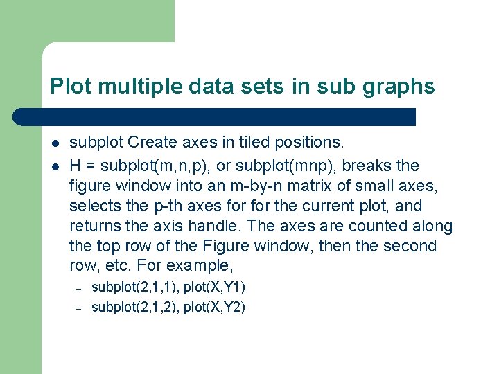
Plot multiple data sets in sub graphs l l subplot Create axes in tiled positions. H = subplot(m, n, p), or subplot(mnp), breaks the figure window into an m-by-n matrix of small axes, selects the p-th axes for the current plot, and returns the axis handle. The axes are counted along the top row of the Figure window, then the second row, etc. For example, – – subplot(2, 1, 1), plot(X, Y 1) subplot(2, 1, 2), plot(X, Y 2)

Plot multiple data sets in sub graphs l subplot('position', [left bottom width height]) creates an axis at the specified position in normalized coordinates (in in the range from 0. 0 to 1. 0). For example subplot(2, 2, [1 3]) plot(X, Y 3) subplot(2, 2, 2) plot(X, Y 1) subplot(2, 2, 4) plot(X, Y 2)

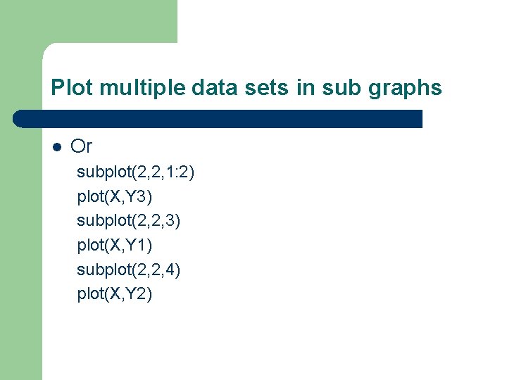
Plot multiple data sets in sub graphs l Or subplot(2, 2, 1: 2) plot(X, Y 3) subplot(2, 2, 3) plot(X, Y 1) subplot(2, 2, 4) plot(X, Y 2)

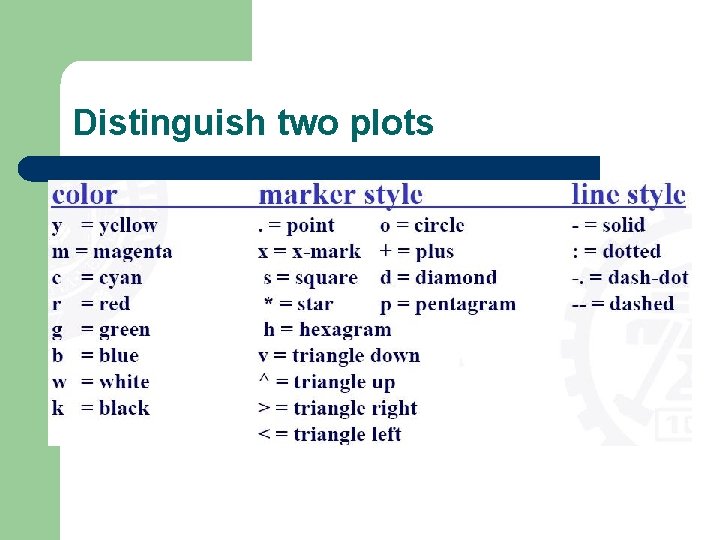
Distinguish two plots

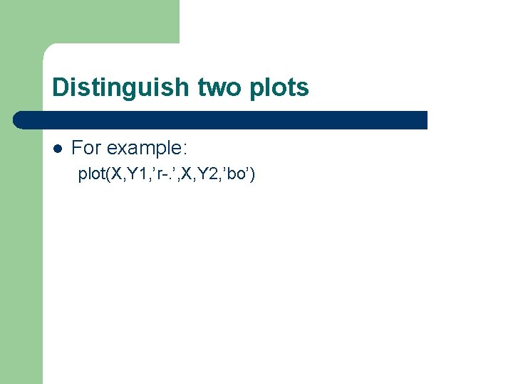
Distinguish two plots l For example: plot(X, Y 1, ’r-. ’, X, Y 2, ’bo’)

Legend l legend(string 1, string 2, string 3. , . . . ) puts a legend on the current plot using the specified strings as labels l legend(H, string 1, string 2, string 3, . . . ) puts a legend on the plot containing the handles in the vector H using the specified strings as labels for the corresponding handles. l legend(AX, . . . ) puts a legend on the axes with handle AX. l legend(M), where M is a string matrix, and LEGEND(H, M) where H is a vector of handles to lines and patches also works. l legend('off') removes the legend from the current axes.

Legend l legend() with no arguments refreshes the current legend, if there is one. If there are multiple legends present, legend(legendhandle) refreshes the specified legend. l legend(. . . , Pos) places the legend in the specified location: – 0 = Automatic "best" placement (least conflict with data) – 1 = Upper right-hand corner (default) – 2 = Upper left-hand corner – 3 = Lower left-hand corner – 4 = Lower right-hand corner – -1 = To the right of the plot

Legend l To move the legend, press the left mouse button on the legend and drag to the desired location. l Legend() works on line graphs, bar graphs, pie graphs, ribbon plots, etc. You can label any solidcolored patch or surface object. l Double clicking on a label allows you to edit the label.

Text l l text(X, Y, 'string') adds the text in the quotes to location (X, Y) on the current axes, where (X, Y) is in units from the current plot. If X and Y are vectors, TEXT writes the text at all locations given. If 'string' is an array the same number of rows as the length of X and Y, TEXT marks each point with the corresponding row of the 'string' array. Example plot(0: pi/20: 2*pi, sin(0: pi/20: 2*pi)) text(pi, 0, ' leftarrow sin(pi)', 'Font. Size', 18)

Print l l Print Figure or model. Save to disk as image or M-file. print: it sends the current figure to your current printer. The size and shape of the printed output depends on the Figure's Paper. Position[mode] properties and your default print command as specified in your PRINTOPT. M file. print filename: it directs the output to the Post. Script file designated by filename. If filename does not include an extension, print appends an appropriate extension. print -dformat filename: it exports the figure to the specified file using the specified graphics format, (such as bmp eps and jpeg).

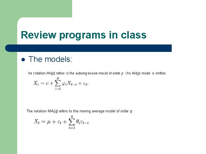
Review programs in class l The models:

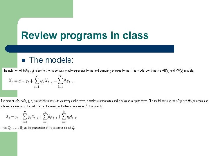
Review programs in class l The models:

Review programs in class l Some functions – round: Round to nearest integer – diff: Differences and approximate derivatives l – diff(x) calculates differences between adjacent elements of X. Load: load filename loads all the variables from the file specified by filename.

l System Identification Toolbox – Estimate linear and nonlinear mathematical models of dynamic systems from measured data. – Simulate output of a system for given input – Predict future outputs on previous observations of inputs and outputs

l Manuals for System Identification Toolbox – – Getting started http: //www. mathworks. com/access/helpdesk/help/ pdf_doc/ident_gs. pdf User guide http: //www. mathworks. com/access/helpdesk/help/ pdf_doc/ident. pdf

Review programs in class l Some functions – idinput: idinput generates input signals of different kinds, which are typically used for identification purposes. u is returned as a matrix or column vector. l – u = idinput(400, 'rbs', [0 0. 3]); 400 is # of data generated. rbs means these random data are from gaussian distribution [0, 0. 03] is the lower and upper bound. poly 2 th: Constructs a "theta-matrix" from given polynomials. l th 0 = poly 2 th(A, B, C); th 0 contains parameters of the equation: A(q) y(t) = B(q) u(t-1) + [C(q)] e(t)

l Some functions – idsim: Simulate systems specified in theta format l y = idsim([u e], th 0); u is data, e is noise, and th 0 is the parameter. – idplot: Plot input-output data. – th 2 ff: Compute the frequency response and standard deviations of a theta format model. – ffplot: Plot frequency response and spectra

Review programs in class l Some functions: – armax: l l – Estimate the parameters of an ARMAX or ARMA model. m = armax(data, orders) returns an idpoly model m with estimated parameters and covariances (parameter uncertainties). Estimates the parameters using the prediction-error method and specified orders. th 1 = armax([y u], [2 2 2 1]); [y, u] is data. [2 2 2 1]is order. The first three is the order of parameters and the last one is for lag (or delay) bodeplot: Plot Bode frequency response and return plot handle. l A Bode plot is a graph of the logarithm of the transfer function of a linear, time-invariant system versus frequency, plotted with a logfrequency axis, to show the system's frequency response.

Useful materials for matlab l Econometrics Toolbox: by James P. Le. Sage – l http: //www. spatial-econometrics. com/ UCSD GARCH – http: //www. kevinsheppard. com/wiki/UCSD_GA RCH