Turing Machines 13 5 Longin Jan Latecki Temple

Turing Machines (13. 5) Longin Jan Latecki Temple University Based on slides by Costas Busch from the course http: //www. cs. rpi. edu/courses/spring 05/modcomp/ and … 1

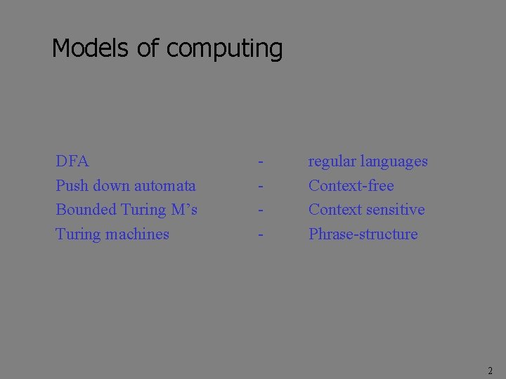
Models of computing DFA Push down automata Bounded Turing M’s Turing machines - regular languages Context-free Context sensitive Phrase-structure 2

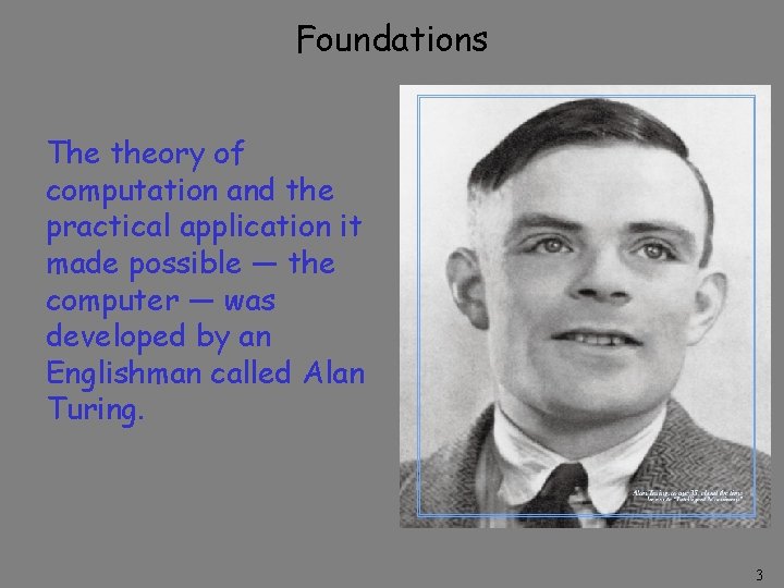
Foundations The theory of computation and the practical application it made possible — the computer — was developed by an Englishman called Alan Turing. 3

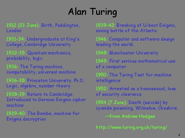
Alan Turing 1912 (23 June): Birth, Paddington, London 1939 -42: Breaking of U-boat Enigma, saving battle of the Atlantic 1931 -34: Undergraduate at King's College, Cambridge University 1946: Computer and software design leading the world. 1932 -35: Quantum mechanics, probability, logic 1948: Manchester University 1936: The Turing machine, computability, universal machine 1936 -38: Princeton University. Ph. D. Logic, algebra, number theory 1938 -39: Return to Cambridge. Introduced to German Enigma cipher machine 1939 -40: The Bombe, machine for Enigma decryption 1949: First serious mathematical use of a computer 1950: The Turing Test for machine intelligence 1952: Arrested as a homosexual, loss of security clearance 1954 (7 June): Death (suicide) by cyanide poisoning, Wilmslow, Cheshire. —from Andrew Hodges http: //www. turing. org. uk/turing/ 4

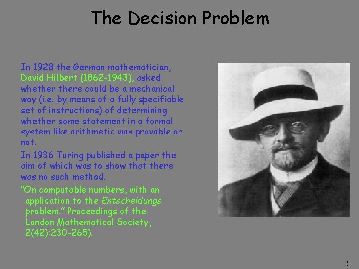
The Decision Problem In 1928 the German mathematician, David Hilbert (1862 -1943), asked whethere could be a mechanical way (i. e. by means of a fully specifiable set of instructions) of determining whether some statement in a formal system like arithmetic was provable or not. In 1936 Turing published a paper the aim of which was to show that there was no such method. “On computable numbers, with an application to the Entscheidungs problem. ” Proceedings of the London Mathematical Society, 2(42): 230 -265). 5

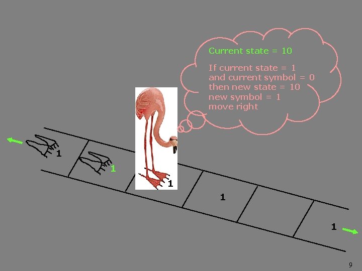
The Turing Machine In order to argue for this claim, he needed a clear concept of “mechanical procedure. ” His idea — which came to be called the Turing machine — was this: (1) A tape of infinite length (2) Finitely many squares of the tape have a single symbol from a finite language. (3) Someone (or something) that can read the squares and write in them. (4) At any time, the machine is in one of a finite number of internal states. (5) The machine has instructions that determine what it does given its internal state and the symbol it encounters on the tape. It can change its internal state; change the symbol on the square; move forward; move backward; halt (i. e. stop). 6

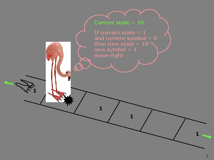
Current state = 10 If current state = 1 and current symbol = 0 then new state = 10 new symbol = 1 move right 1 0 1 1 1 7

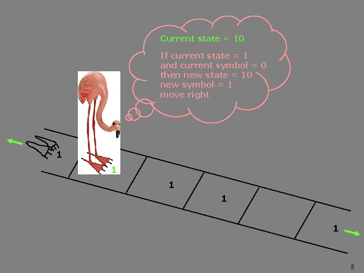
Current state = 10 If current state = 1 and current symbol = 0 then new state = 10 new symbol = 1 move right 1 1 1 8

Current state = 10 If current state = 1 and current symbol = 0 then new state = 10 new symbol = 1 move right 1 1 1 9

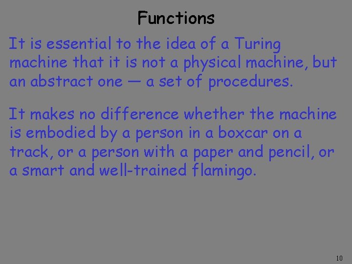
Functions It is essential to the idea of a Turing machine that it is not a physical machine, but an abstract one — a set of procedures. It makes no difference whether the machine is embodied by a person in a boxcar on a track, or a person with a paper and pencil, or a smart and well-trained flamingo. 10

Turing’s Theorem In the 1936 paper Turing proved that there are “generalpurpose” Turing machines that can compute whatever any other Turing machine. This is done by coding the function of the special-purpose machine as instructions of the other machine — that is by “programming” it. This is called Turing’s theorem. These are universal Turing machines, and the idea of a coding for a particular function fed into a universal Turing machine is basically our conception of a computer and a stored program. The concept of the universal Turing machine is just the concept of the computer as we know it. 11

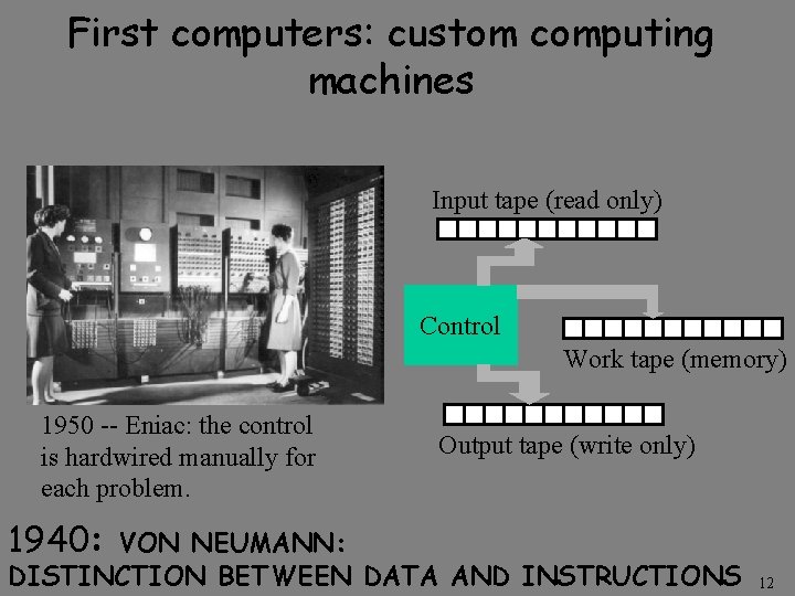
First computers: custom computing machines Input tape (read only) Control Work tape (memory) 1950 -- Eniac: the control is hardwired manually for each problem. Output tape (write only) 1940: VON NEUMANN: DISTINCTION BETWEEN DATA AND INSTRUCTIONS 12

Can Machines Think? In “Computing machinery and intelligence, ” written in 1950, Turing asks whether machines can think. He claims that this question is too vague, and proposes, instead, to replace it with a different one. That question is: Can machines pass the “imitation game” (now called the Turing test)? If they can, they are intelligent. Turing is thus the first to have offered a rigorous test for the determination of intelligence quite generally. 13

The Turing Test The game runs as follows. You sit at a computer terminal and have an electronic conversation. You don’t know who is on the other end; it could be a person or a computer responding as it has been programmed to do. If you can’t distinguish between a human being and a computer from your interactions, then the computer is intelligent. Note that this is meant to be a sufficient condition of intelligence only. There may be other ways to be intelligent. 14

Artificial Intelligence 15

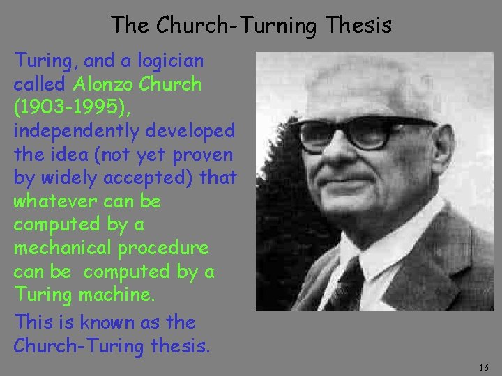
The Church-Turning Thesis Turing, and a logician called Alonzo Church (1903 -1995), independently developed the idea (not yet proven by widely accepted) that whatever can be computed by a mechanical procedure can be computed by a Turing machine. This is known as the Church-Turing thesis. 16

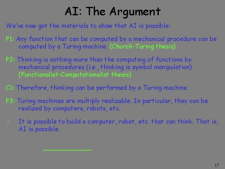
AI: The Argument We’ve now got the materials to show that AI is possible: P 1: Any function that can be computed by a mechanical procedure can be computed by a Turing machine. (Church-Turing thesis) P 2: Thinking is nothing more than the computing of functions by mechanical procedures (i. e. , thinking is symbol manipulation). (Functionalist-Computationalist thesis) C 1: Therefore, thinking can be performed by a Turing machine. P 3: Turing machines are multiply realizable. In particular, they can be realized by computers, robots, etc. It is possible to build a computer, robot, etc. that can think. That is, AI is possible. 17

Turing Machines 18

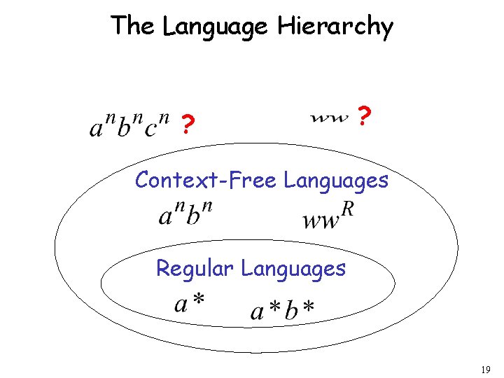
The Language Hierarchy ? ? Context-Free Languages Regular Languages 19

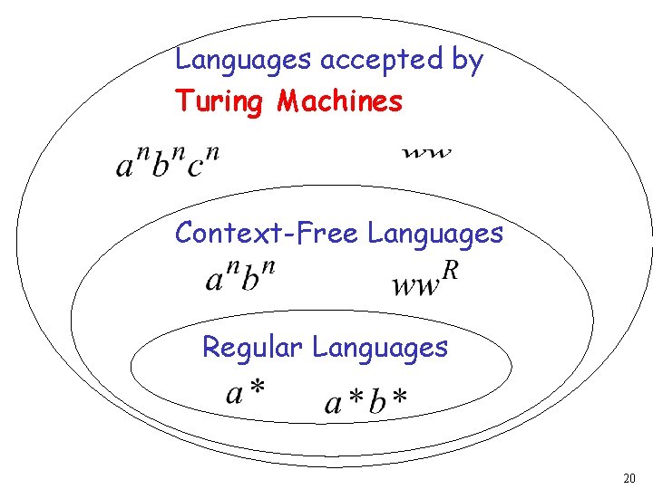
Languages accepted by Turing Machines Context-Free Languages Regular Languages 20

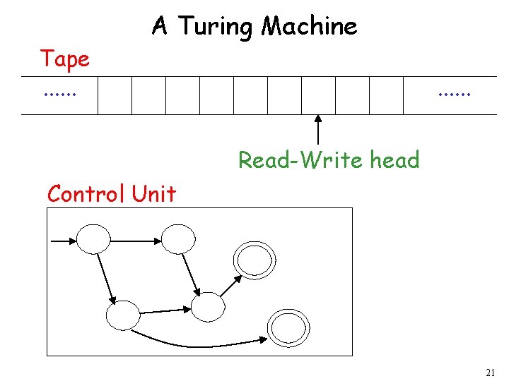
Tape. . . A Turing Machine. . . Read-Write head Control Unit 21

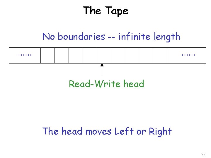
The Tape No boundaries -- infinite length. . . Read-Write head The head moves Left or Right 22

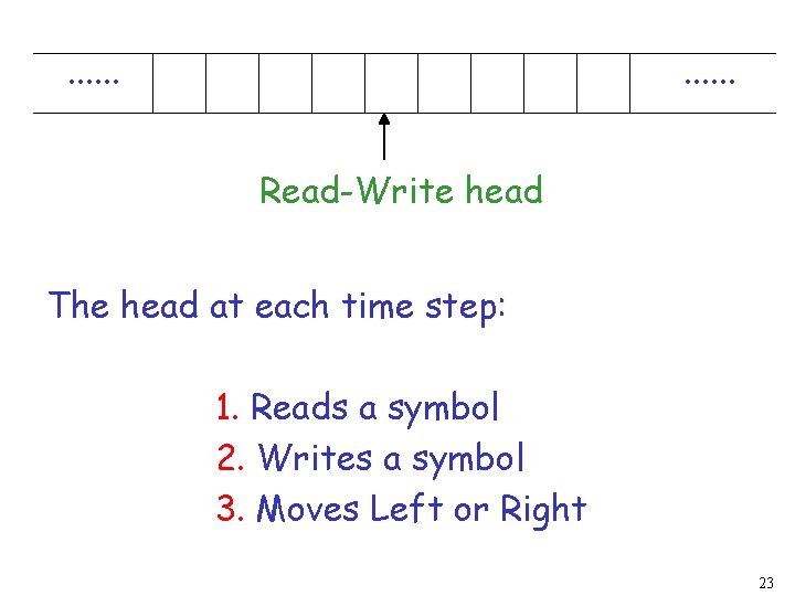
. . . Read-Write head The head at each time step: 1. Reads a symbol 2. Writes a symbol 3. Moves Left or Right 23

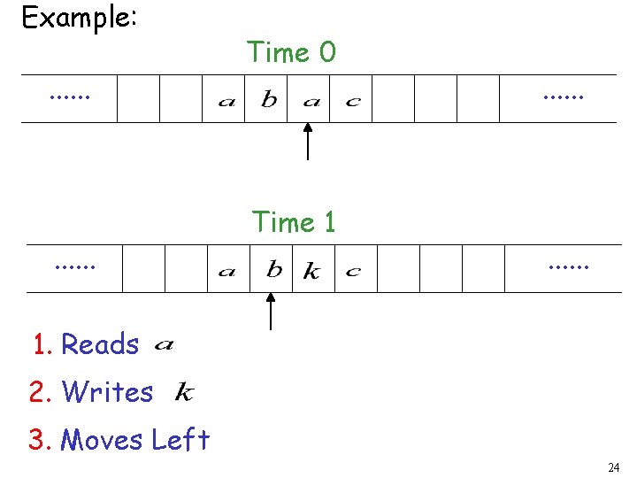
Example: . . . Time 0 Time 1 . . . 1. Reads 2. Writes 3. Moves Left 24

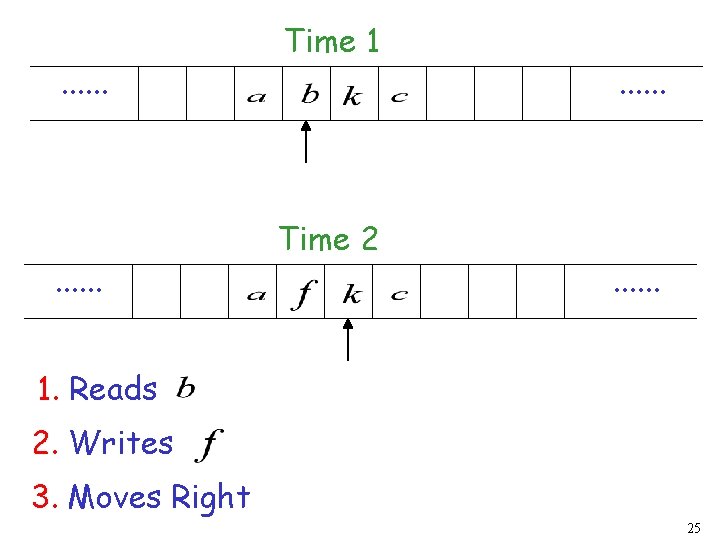
. . . Time 1 Time 2 . . . 1. Reads 2. Writes 3. Moves Right 25

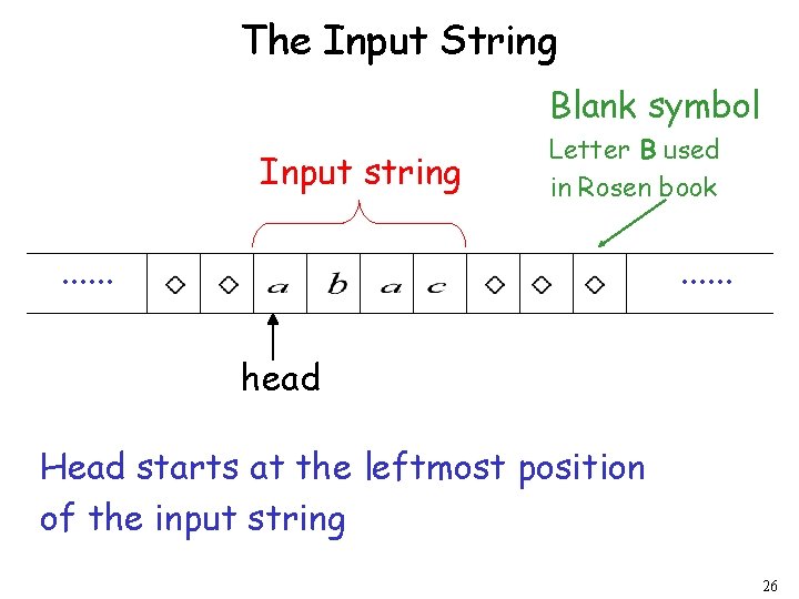
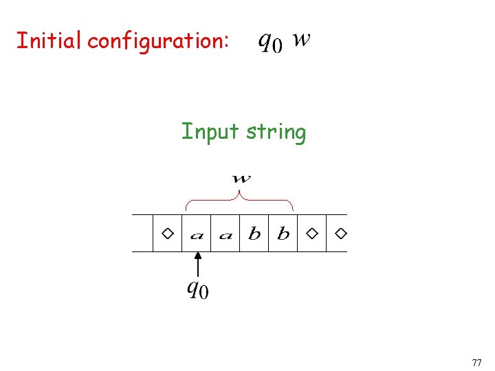
The Input String Blank symbol Input string Letter B used in Rosen book . . . head Head starts at the leftmost position of the input string 26

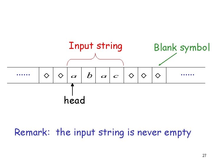
Input string. . . Blank symbol. . . head Remark: the input string is never empty 27

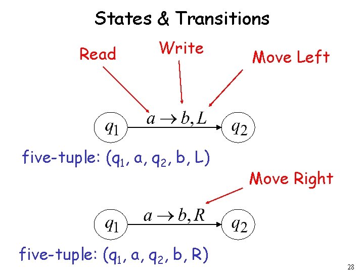
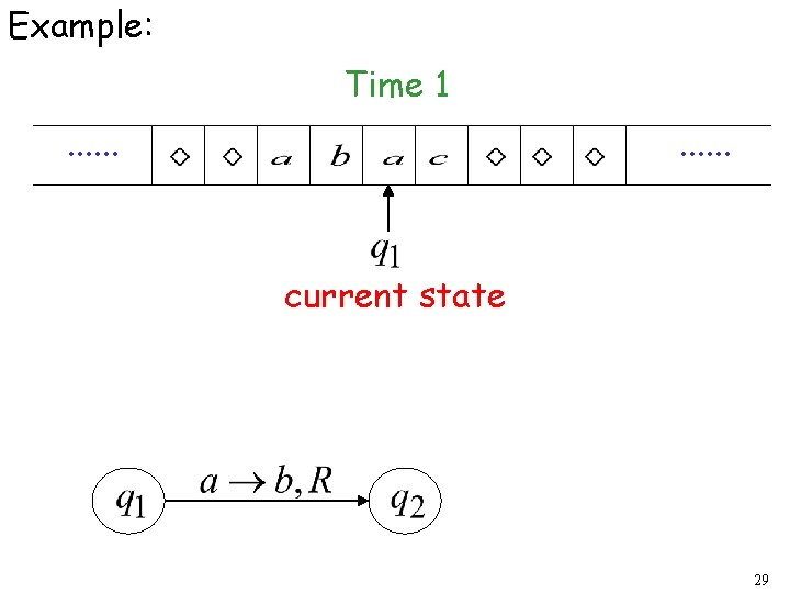
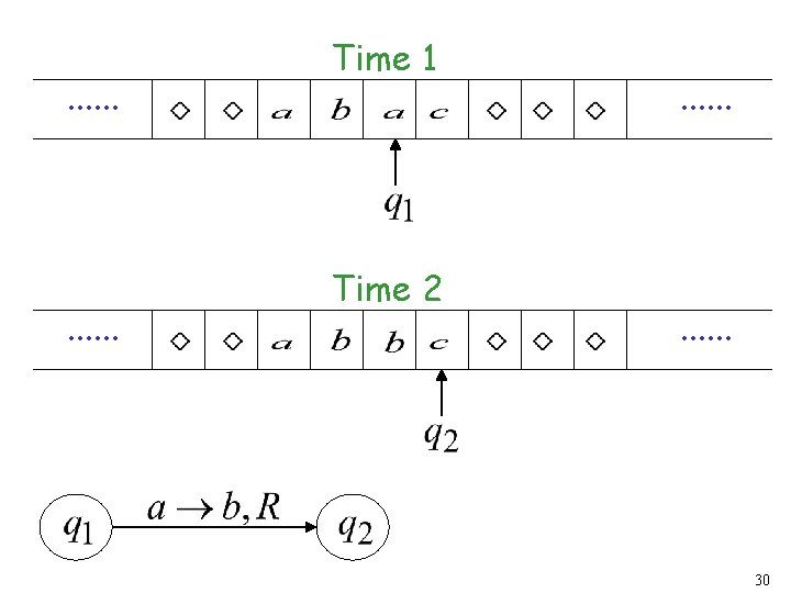
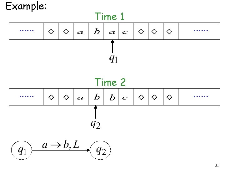
States & Transitions Read Write five-tuple: (q 1, a, q 2, b, L) five-tuple: (q 1, a, q 2, b, R) Move Left Move Right 28

Example: Time 1. . . current state 29

. . . Time 1 Time 2 . . . 30

Example: . . . Time 1 Time 2 . . . 31

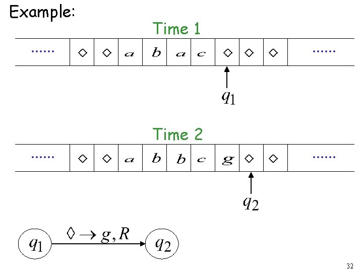
Example: . . . Time 1 Time 2 . . . 32

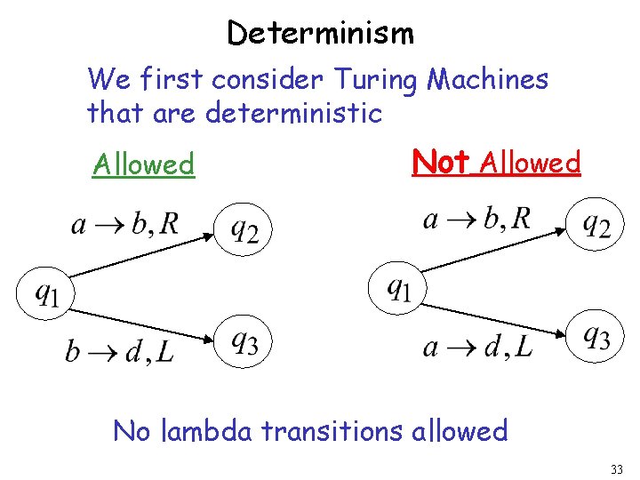
Determinism We first consider Turing Machines that are deterministic Allowed Not Allowed No lambda transitions allowed 33

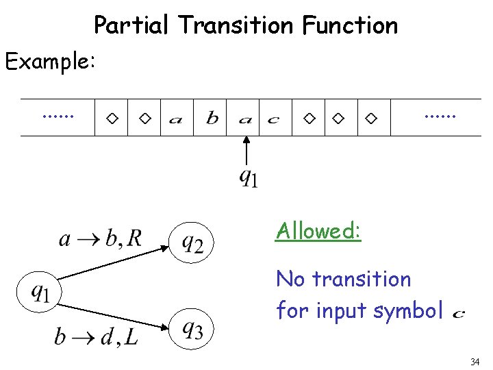
Partial Transition Function Example: . . . Allowed: No transition for input symbol 34

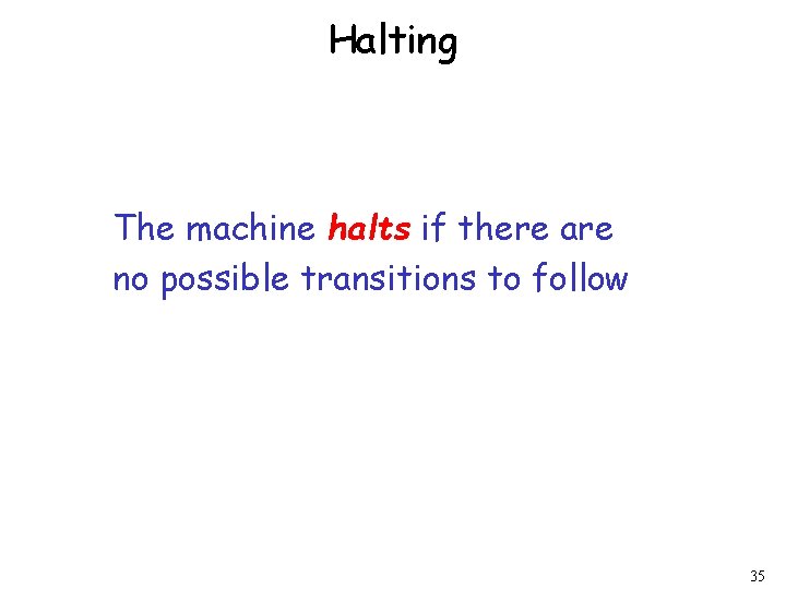
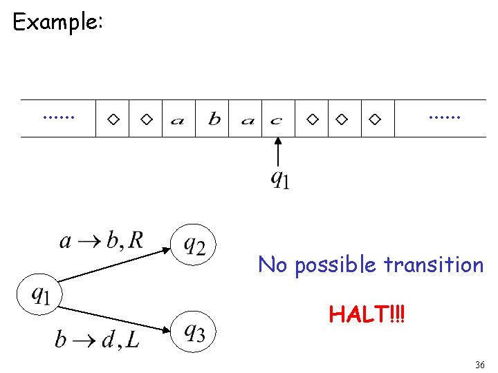
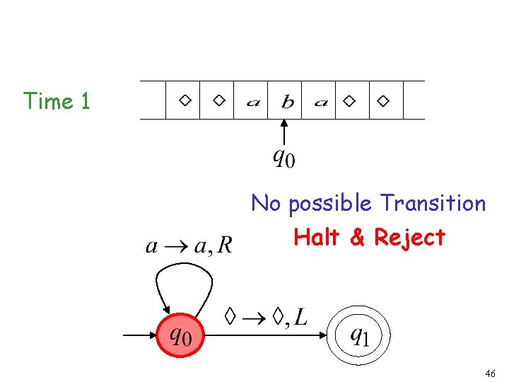
Halting The machine halts if there are no possible transitions to follow 35

Example: . . . No possible transition HALT!!! 36

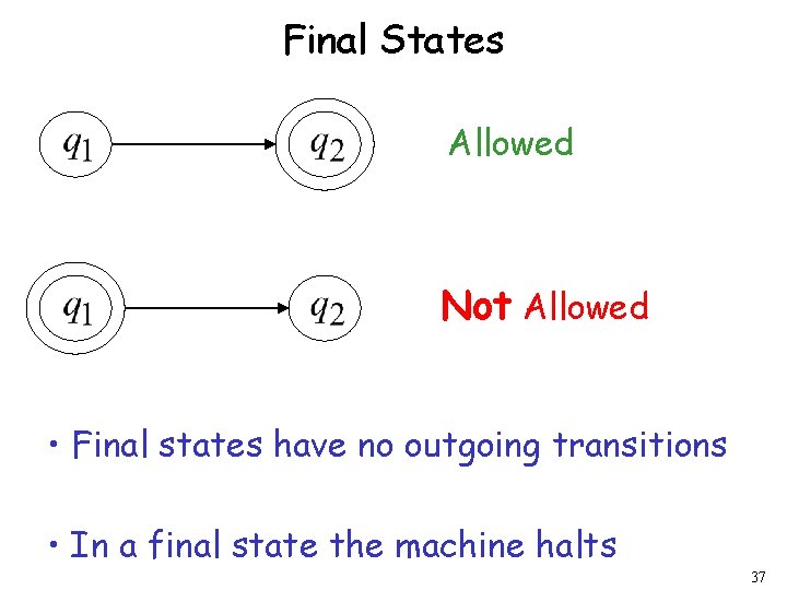
Final States Allowed Not Allowed • Final states have no outgoing transitions • In a final state the machine halts 37

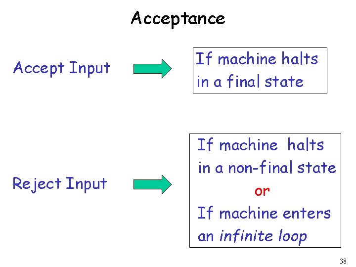
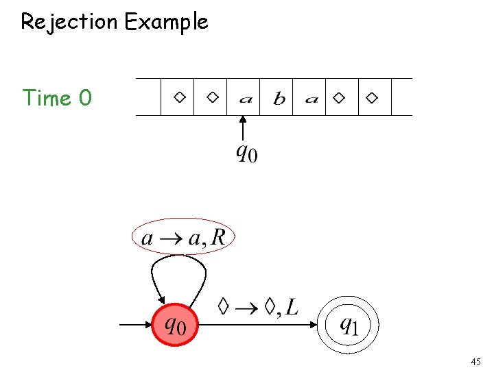
Acceptance Accept Input If machine halts in a final state Reject Input If machine halts in a non-final state or If machine enters an infinite loop 38

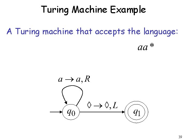
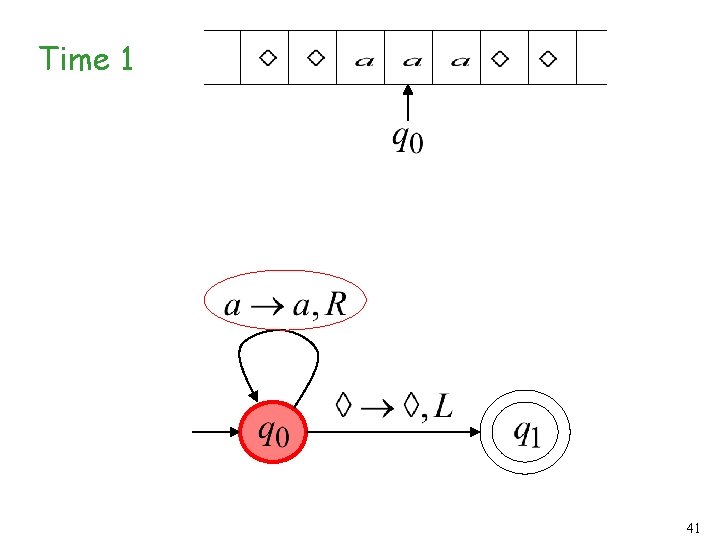
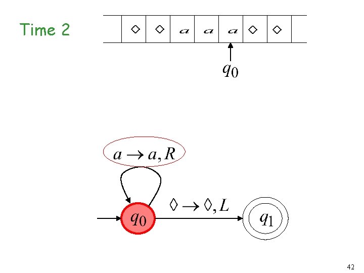
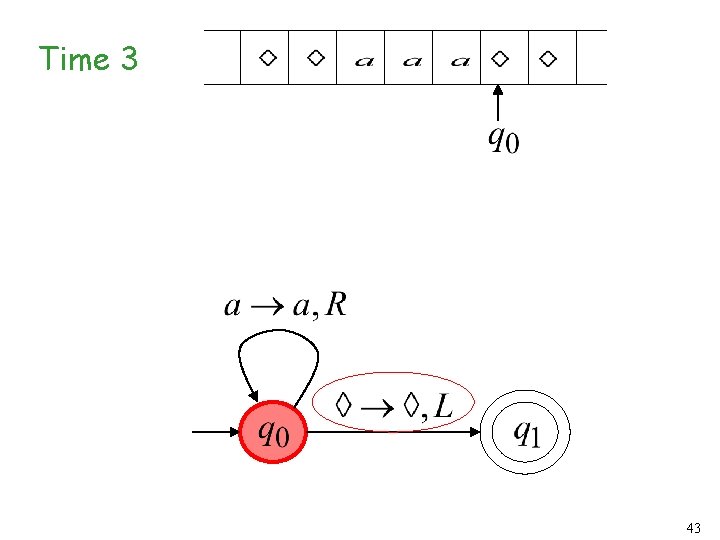
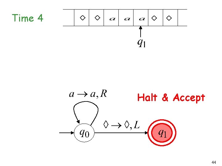
Turing Machine Example A Turing machine that accepts the language: 39

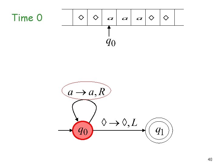
Time 0 40

Time 1 41

Time 2 42

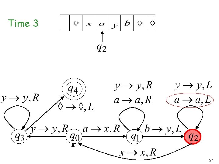
Time 3 43

Time 4 Halt & Accept 44

Rejection Example Time 0 45

Time 1 No possible Transition Halt & Reject 46

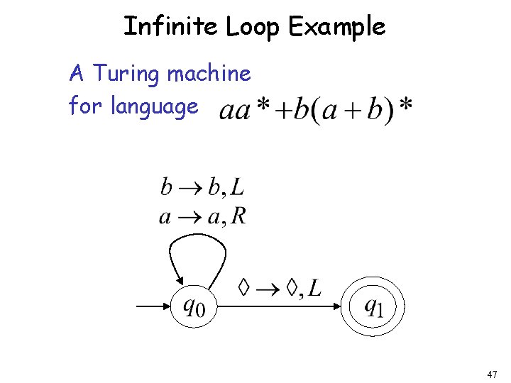
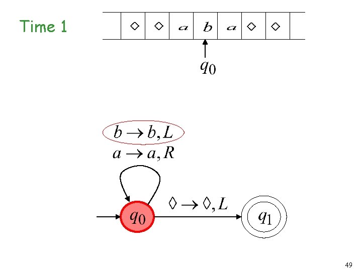
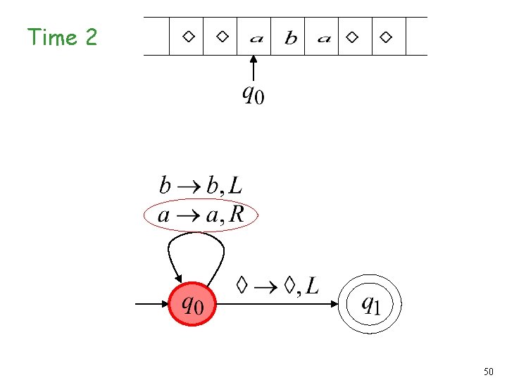
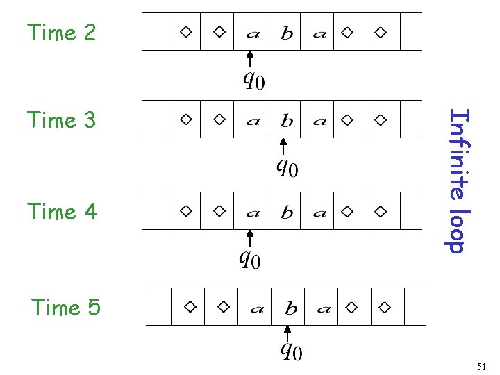
Infinite Loop Example A Turing machine for language 47

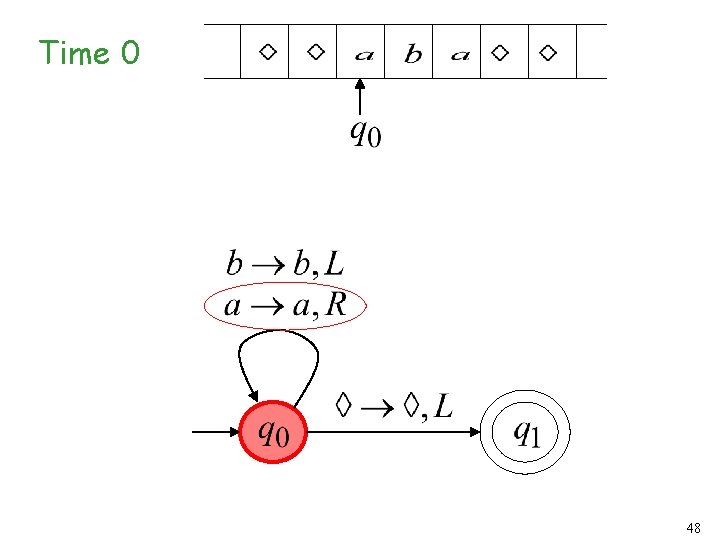
Time 0 48

Time 1 49

Time 2 50

Time 2 Time 4 Infinite loop Time 3 Time 5 51

Because of the infinite loop: • The final state cannot be reached • The machine never halts • The input is not accepted 52

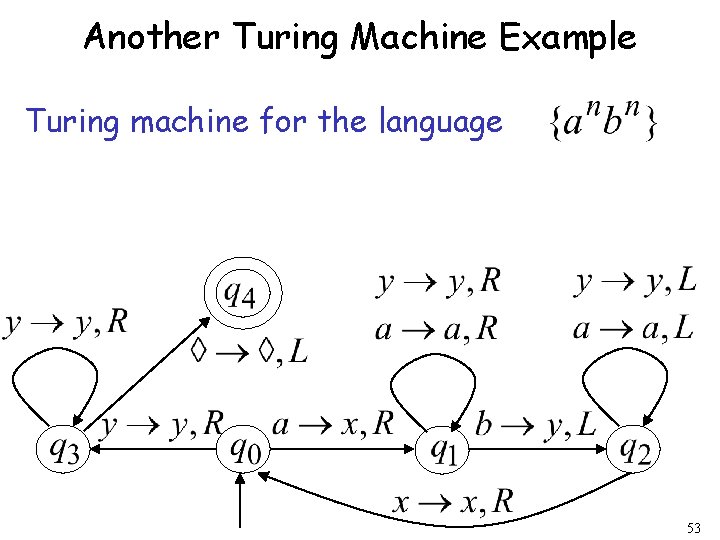
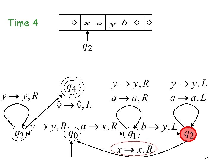
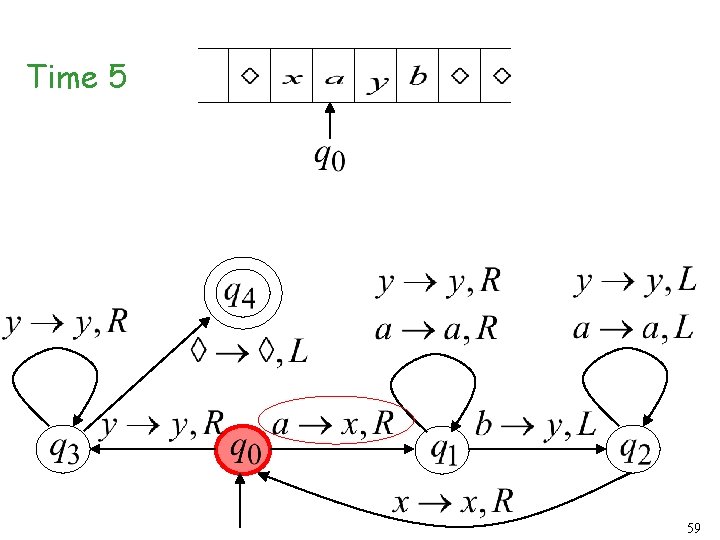
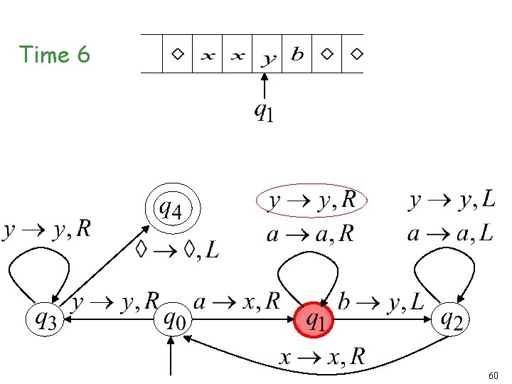
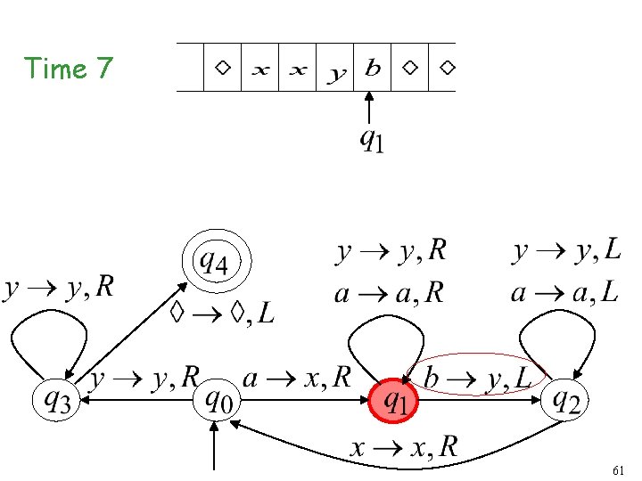
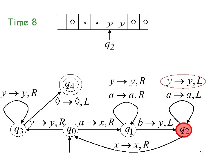
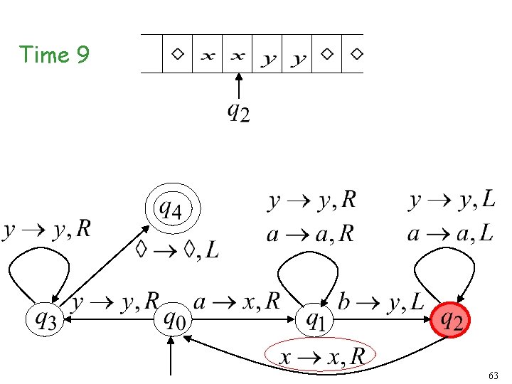
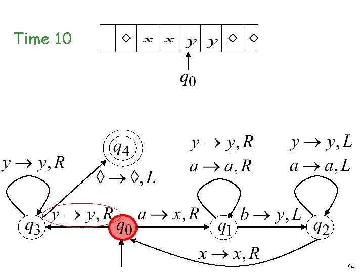
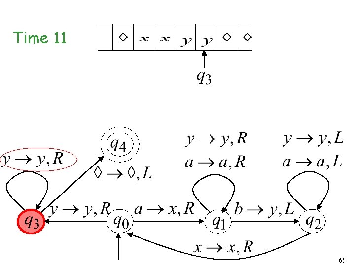
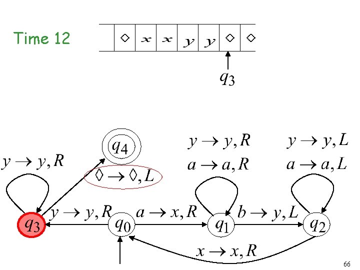
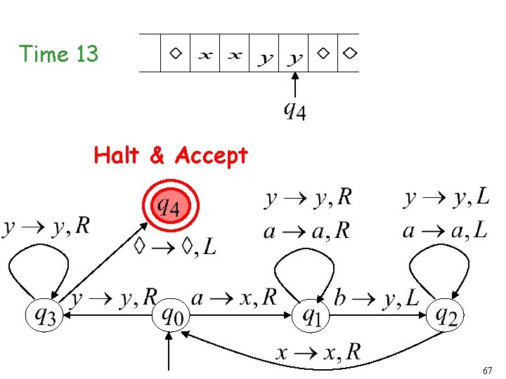
Another Turing Machine Example Turing machine for the language 53

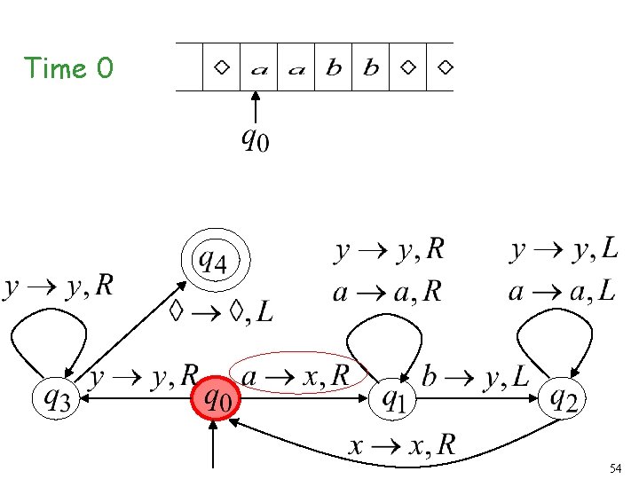
Time 0 54

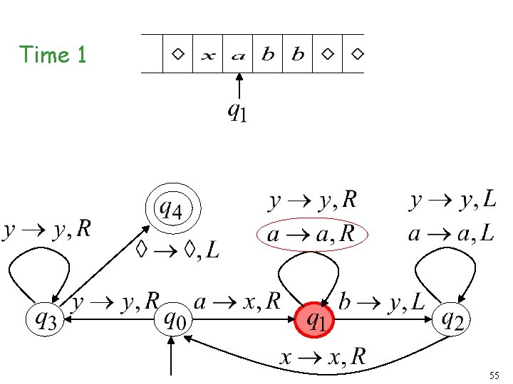
Time 1 55

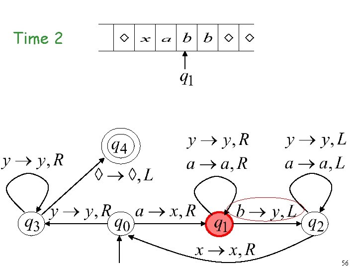
Time 2 56

Time 3 57

Time 4 58

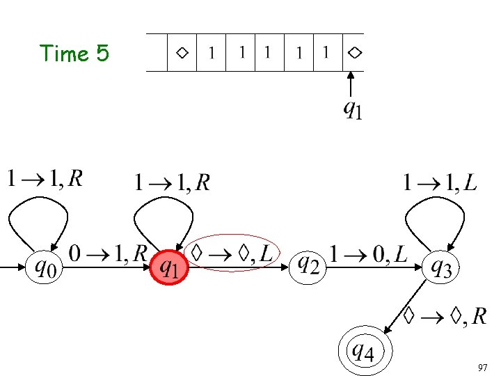
Time 5 59

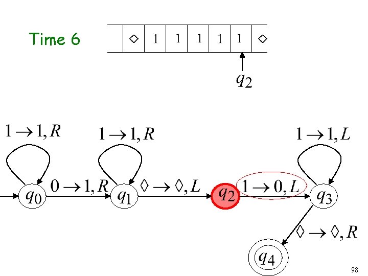
Time 6 60

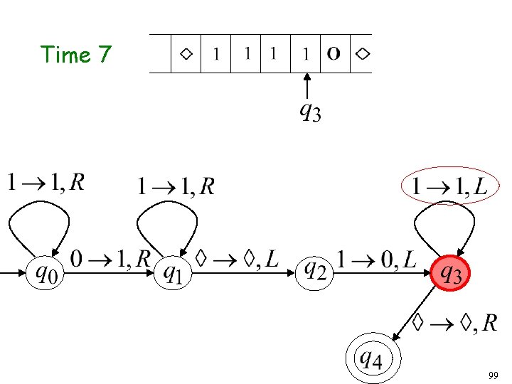
Time 7 61

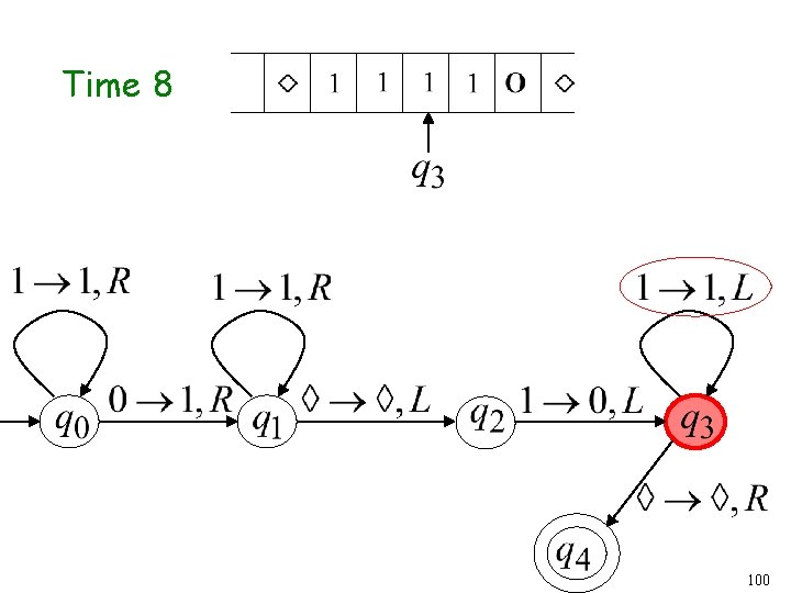
Time 8 62

Time 9 63

Time 10 64

Time 11 65

Time 12 66

Time 13 Halt & Accept 67

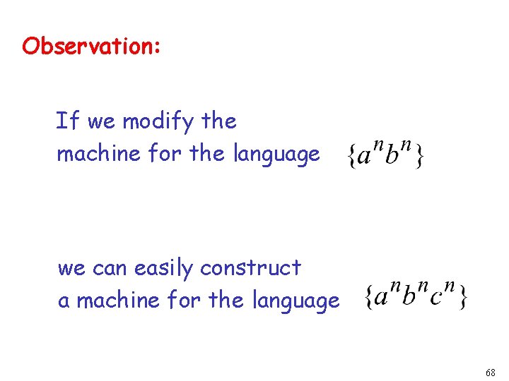
Observation: If we modify the machine for the language we can easily construct a machine for the language 68

Formal Definitions for Turing Machines 69

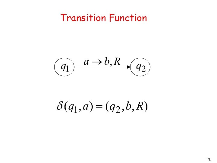
Transition Function 70

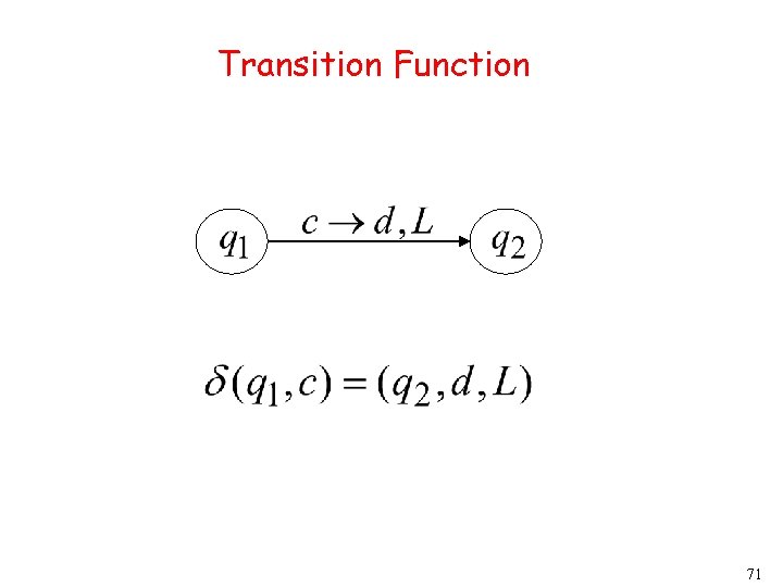
Transition Function 71

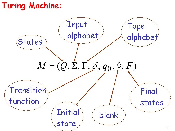
Turing Machine: States Input alphabet Tape alphabet Transition function Initial state Final states blank 72

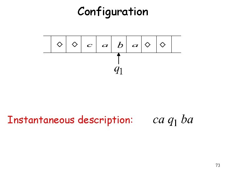
Configuration Instantaneous description: 73

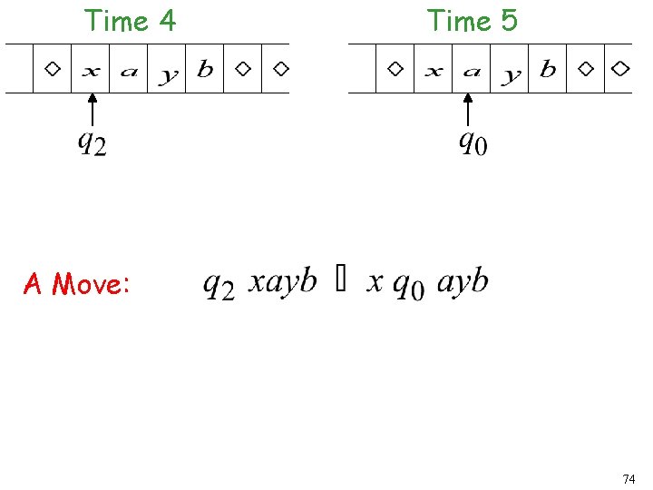
Time 4 Time 5 A Move: 74

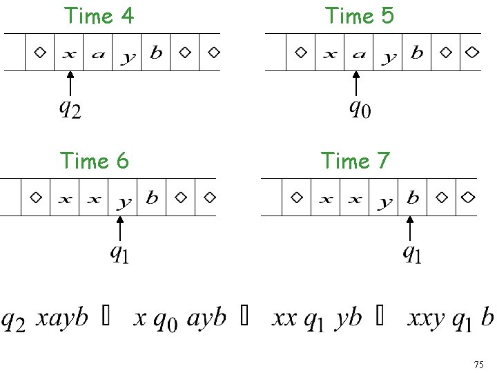
Time 4 Time 5 Time 6 Time 7 75

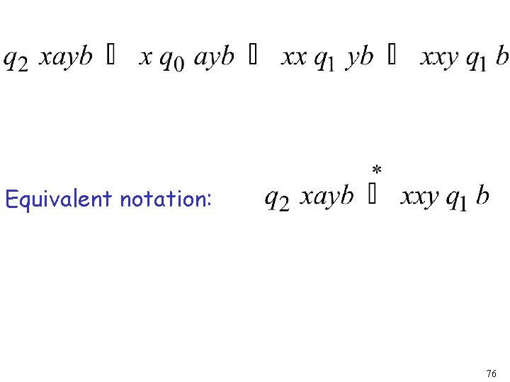
Equivalent notation: 76

Initial configuration: Input string 77

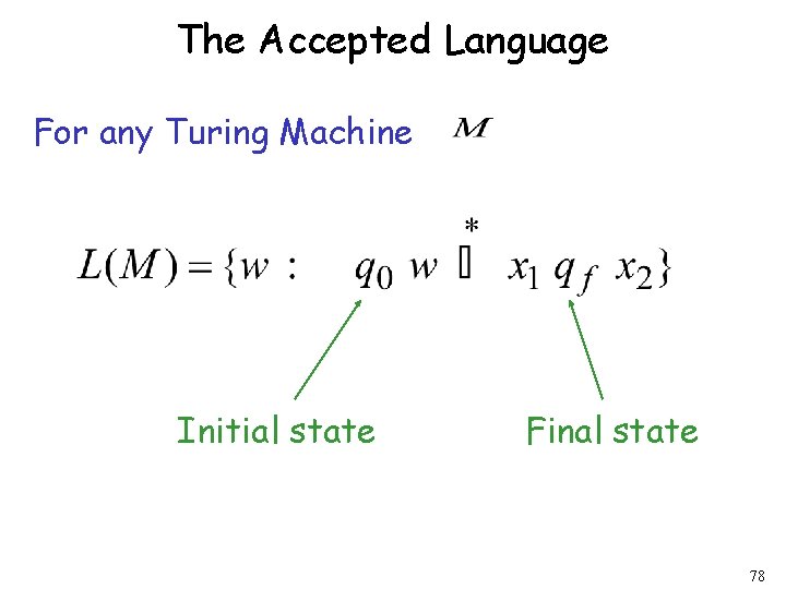
The Accepted Language For any Turing Machine Initial state Final state 78

Standard Turing Machine The machine we described is the standard: • Deterministic • Infinite tape in both directions • Tape is the input/output file 79

Computing Functions with Turing Machines 80

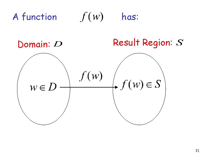
A function Domain: has: Result Region: 81

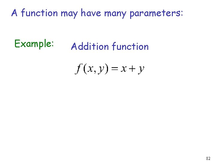
A function may have many parameters: Example: Addition function 82

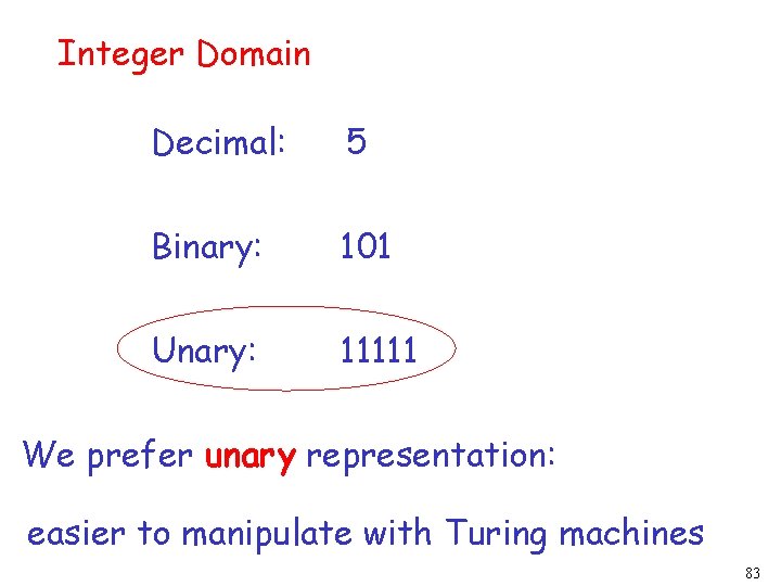
Integer Domain Decimal: 5 Binary: 101 Unary: 11111 We prefer unary representation: easier to manipulate with Turing machines 83

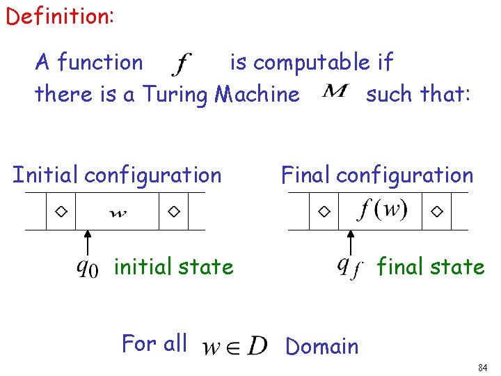
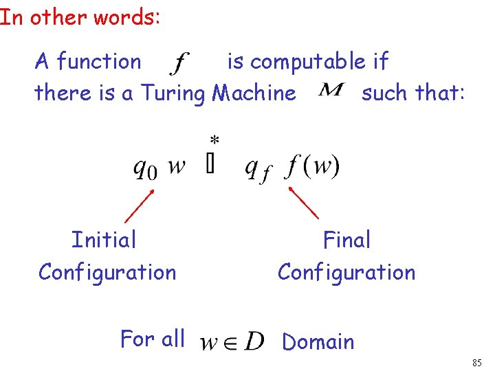
Definition: A function is computable if there is a Turing Machine such that: Initial configuration Final configuration initial state For all final state Domain 84

In other words: A function is computable if there is a Turing Machine such that: Initial Configuration For all Final Configuration Domain 85

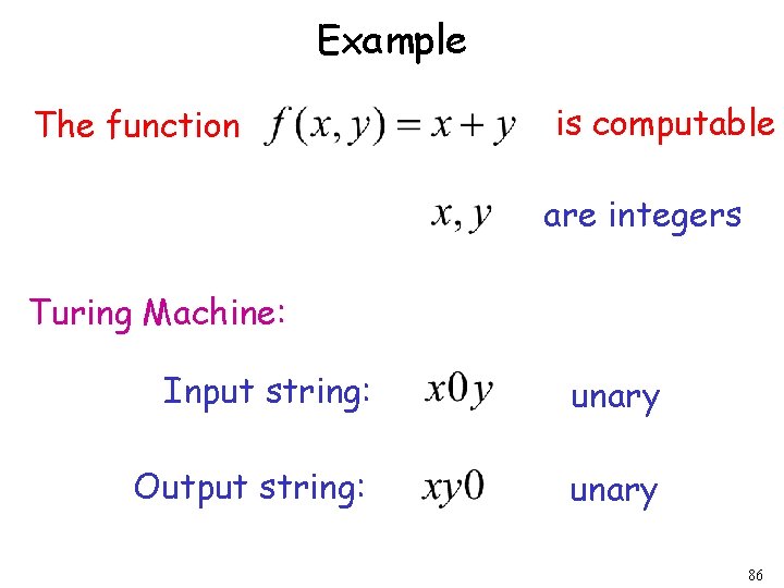
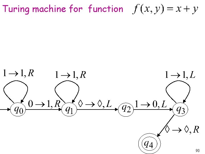
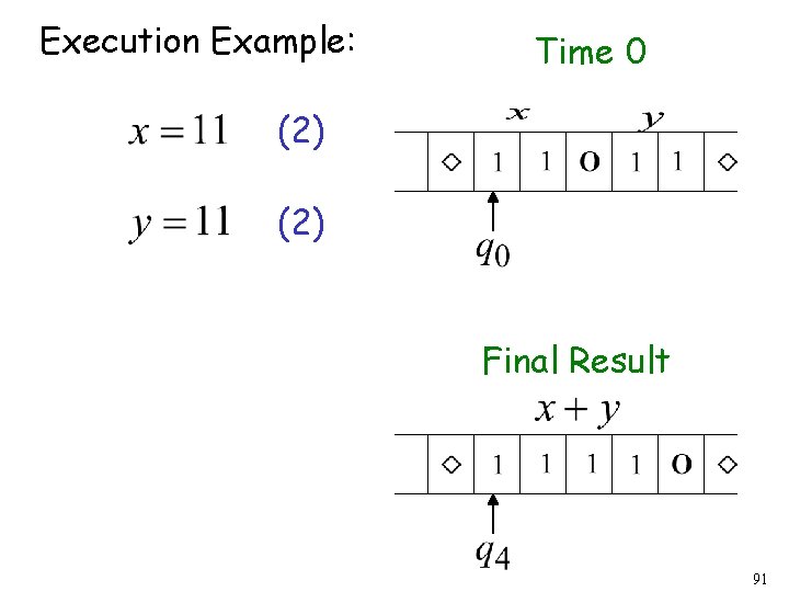
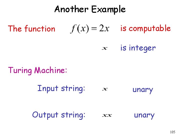
Example The function is computable are integers Turing Machine: Input string: unary Output string: unary 86

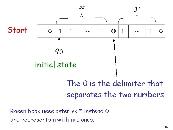
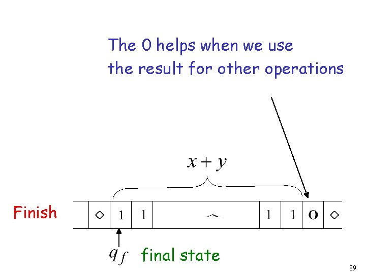
Start initial state The 0 is the delimiter that separates the two numbers Rosen book uses asterisk * instead 0 and represents n with n+1 ones. 87

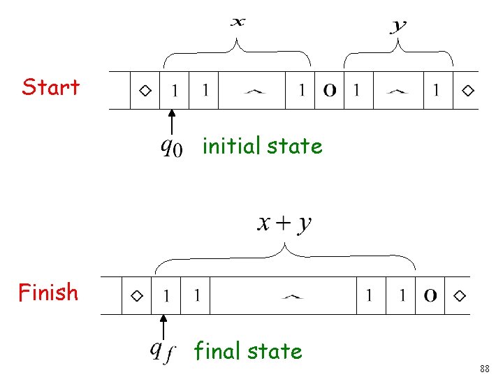
Start initial state Finish final state 88

The 0 helps when we use the result for other operations Finish final state 89

Turing machine for function 90

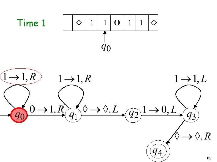
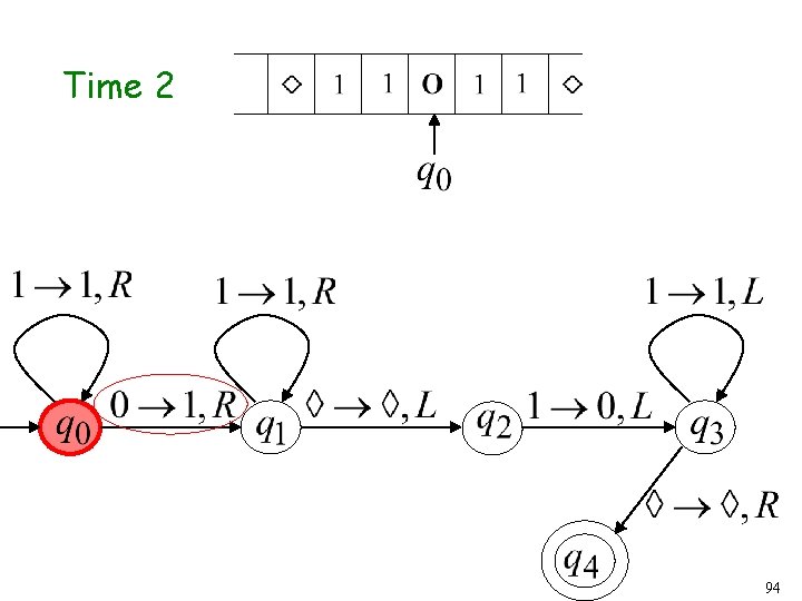
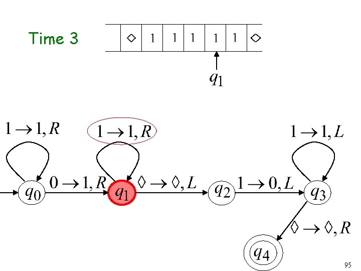
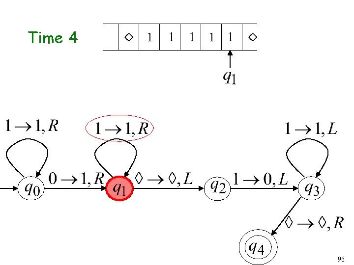
Execution Example: Time 0 (2) Final Result 91

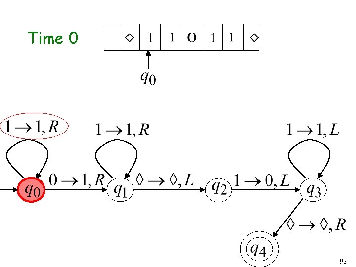
Time 0 92

Time 1 93

Time 2 94

Time 3 95

Time 4 96

Time 5 97

Time 6 98

Time 7 99

Time 8 100

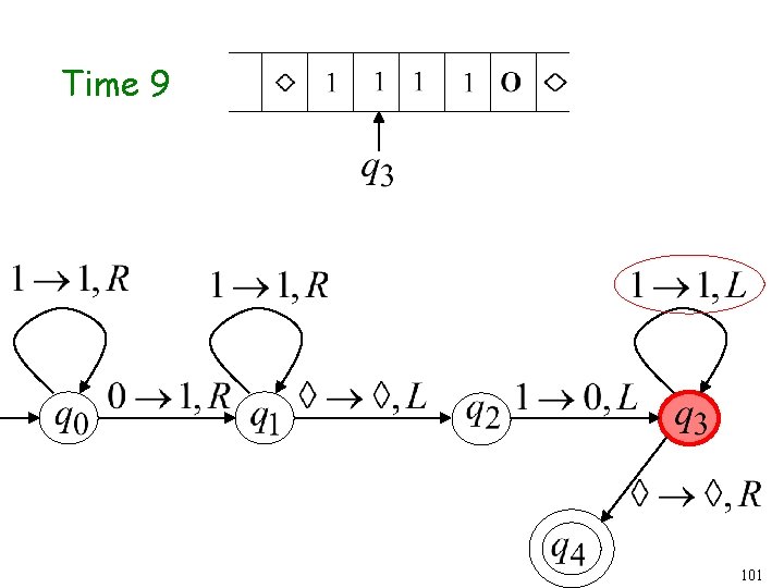
Time 9 101

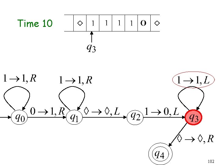
Time 10 102

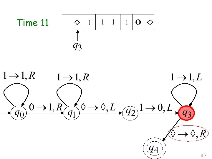
Time 11 103

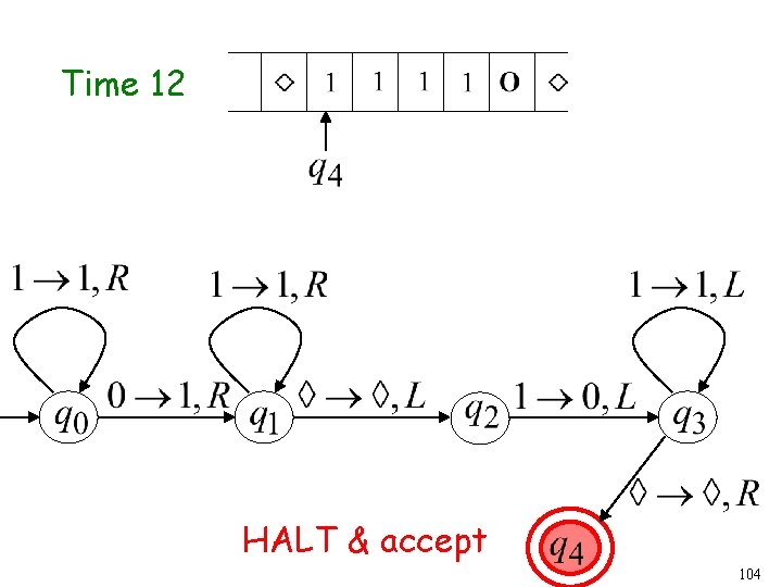
Time 12 HALT & accept 104

Another Example The function is computable is integer Turing Machine: Input string: unary Output string: unary 105

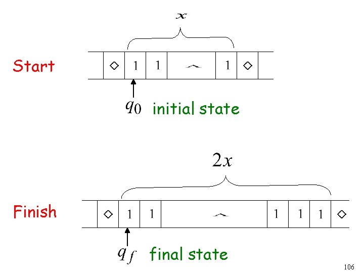
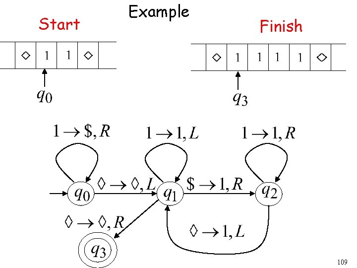
Start initial state Finish final state 106

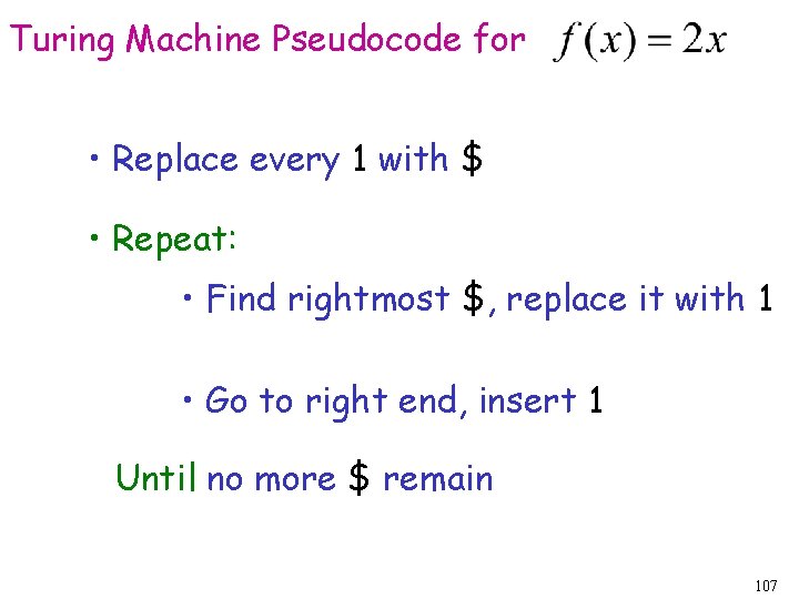
Turing Machine Pseudocode for • Replace every 1 with $ • Repeat: • Find rightmost $, replace it with 1 • Go to right end, insert 1 Until no more $ remain 107

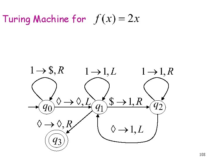
Turing Machine for 108

Start Example Finish 109

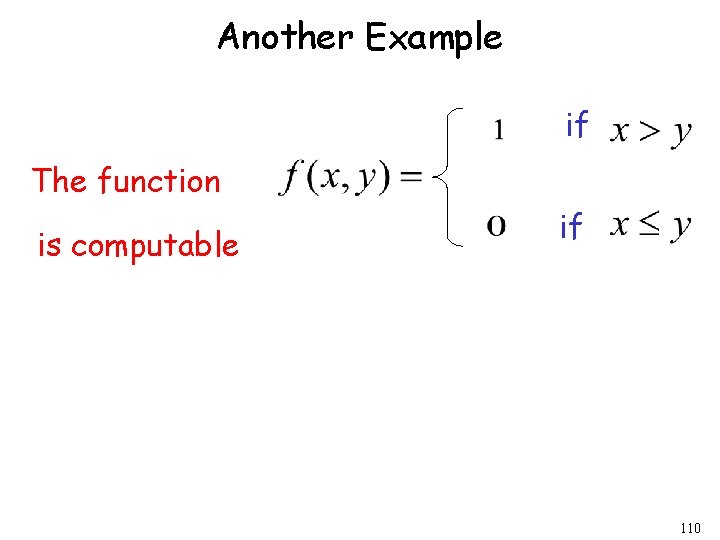
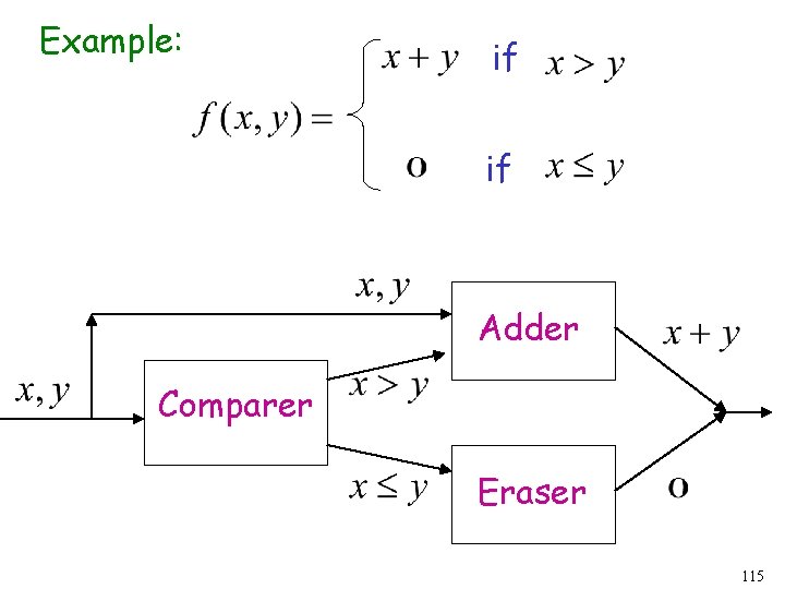
Another Example if The function is computable if 110

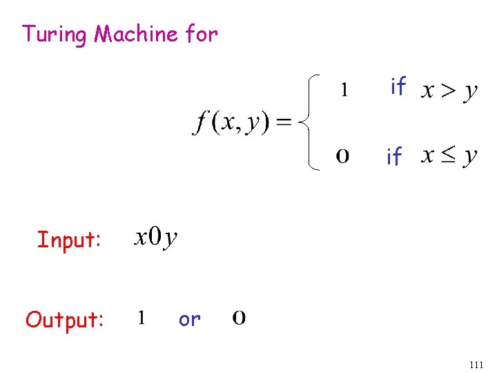
Turing Machine for if if Input: Output: or 111

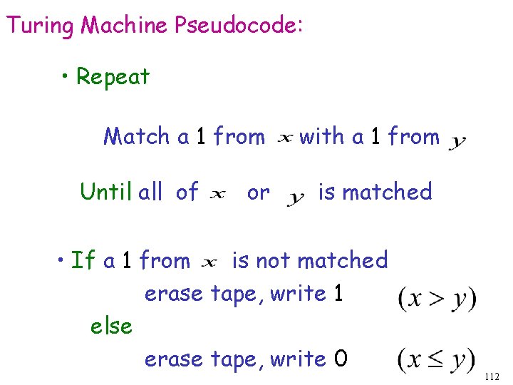
Turing Machine Pseudocode: • Repeat Match a 1 from Until all of or with a 1 from is matched • If a 1 from is not matched erase tape, write 1 else erase tape, write 0 112

Combining Turing Machines 113

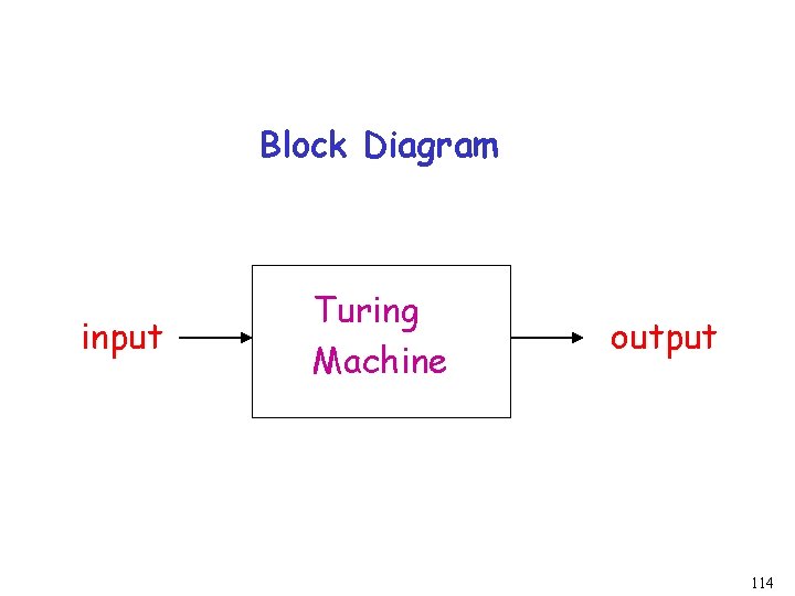
Block Diagram input Turing Machine output 114

Example: if if Adder Comparer Eraser 115

Computational complexity The Turing machines we have studied have all been deterministic, i. e. , when the transition rules are represented as five-tuples (s, x, s’, x’, d), were s, x are the current state and tape symbol, s’, x’ are the next state and tape symbol, and d is the move direction, then no two transition rules begin with the same pair (s, x), i. e. , the mapping (s, x) → (s’, x’, d) is a function. In a nondeterministic Turing machine there maybe more that one transition rule beginning with the same pair (s, x). 116

Decision problem A decision problem asks whether statements from a particular class of statements are true. Decision problems are also known as yes-or-no problems. When there is an effective algorithm that decides whether instances of a decision problem are true, we say that this problem is solvable or decidable The halting problem is the decision problem that asks whether a Turing machine T eventually halts when given an input string x. The halting problem is an unsolvable decision problem. That is, no Turing machine exists that, when given an encoding of a Turing machine T and its input string x as input, can determine whether T eventually halts when started with x written on its tape (proof in Section 3. 1). 117

P class of decision problems A decision problem is in class P of polynomial-time problems if it can be solved by a deterministic Turing machine in a polynomial time as function of the size of the input string, i. e. , there is a deterministic Turing machine T that solves the problem and halts in a final state after no more than p(n) transitions when the input to T is a string of length n. Problems in P are called tractable while problems not in P are called intractable. 118

Examples of tractable problems: (1) determining whether an item is in a list of n elements, (2) determining whether a given positive integer n is prime is tractable (this fact was only proven in 2002!). 119

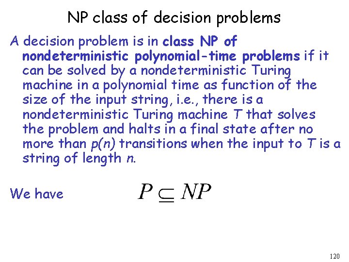
NP class of decision problems A decision problem is in class NP of nondeterministic polynomial-time problems if it can be solved by a nondeterministic Turing machine in a polynomial time as function of the size of the input string, i. e. , there is a nondeterministic Turing machine T that solves the problem and halts in a final state after no more than p(n) transitions when the input to T is a string of length n. We have 120

P and NP One of the most challenging questions in computer science is whether P = NP, i. e. , whether every problem in P is also in NP. A problem S is NP-complete if it belongs to NP and if S can be shown to belong to P then every problem in NP must also belong to P, i. e. , the existence of polynomial-time algorithm to solve S, implies the existence of a polynomial-time algorithm for every problem in NP. Examples of NP-complete problems: (1) whether a simple graph has a Hamilton circuit (a simple circuit that passes through every vertex exactly once) and (2) whether a proposition in n-variables is a tautology. 121