Turbulence in Magnetised Plasma of Galaxies and Clusters

Turbulence in Magnetised Plasma of Galaxies and Clusters Alexander Schekochihin (DAMTP/Cambridge) with Steve Cowley (UCLA), Russell Kulsrud (Princeton), Greg Hammett (Princeton), Sam Taylor (Imperial), Jason Maron (AMNH), Jim Mc. Williams (UCLA) Reprints/references on http: //www. damtp. cam. ac. uk/user/as 629 and on the desk in the back of the room

This is a cluster of galaxies… The Coma Cluster © NASA

This is a galaxy… M 51 The Whirlpool Galaxy © NOAO/AURA/NSF

…and this is the Matrix N 3 The Periodic Box

MHD Turbulence: The Fundamental Problem

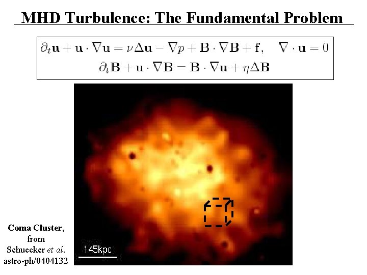
MHD Turbulence: The Fundamental Problem Coma Cluster, from Schuecker et al. astro-ph/0404132

MHD Turbulence: The Fundamental Problem Clusters are wonderful: • amorphous plasma • no rotation (nonhelical!) • subsonic turbulence (from mergers/structure formation) • tangled magnetic fields … a case of “pure” turbulence (more about them later…)

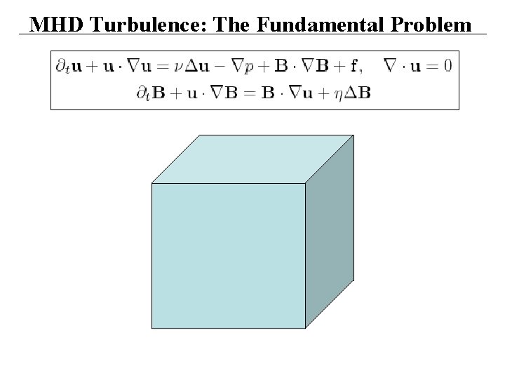
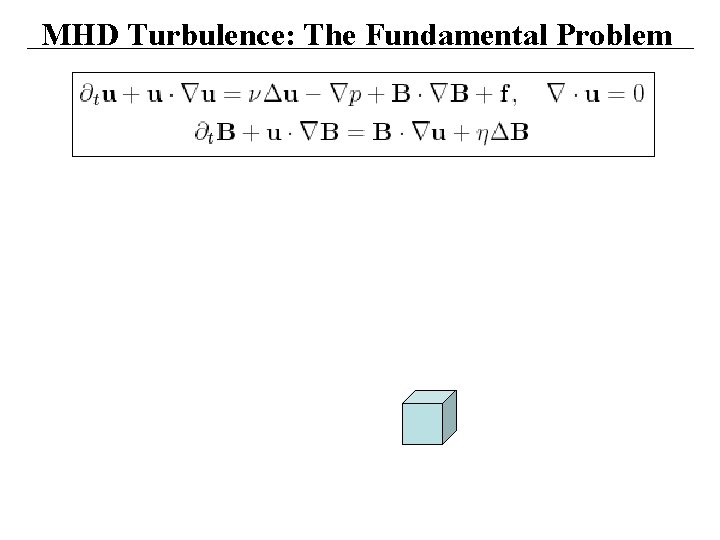
MHD Turbulence: The Fundamental Problem Set B = 0, start with small seed field. There are two main issues: 1. Is there small-scale dynamo, i. e. , does magnetic energy B 2 grow? 2. If it does, how does it saturate: what is the long-term state of the fully-developed isotropic MHD turbulence? Can we simulate this problem in our box? I. e. , what are the scales ranges and what happens at smallest scales?

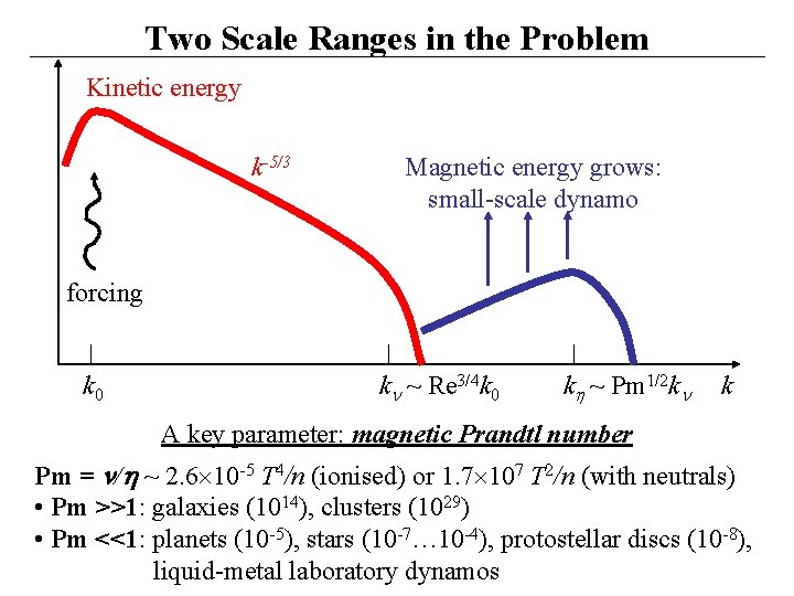
Two Scale Ranges in the Problem Kinetic energy k-5/3 Magnetic energy grows: small-scale dynamo forcing k 0 k ~ Re 3/4 k 0 k ~ Pm 1/2 k k A key parameter: magnetic Prandtl number Pm = / ~ 2. 6 10 -5 T 4/n (ionised) or 1. 7 107 T 2/n (with neutrals) • Pm >>1: galaxies (1014), clusters (1029) • Pm <<1: planets (10 -5), stars (10 -7… 10 -4), protostellar discs (10 -8), liquid-metal laboratory dynamos

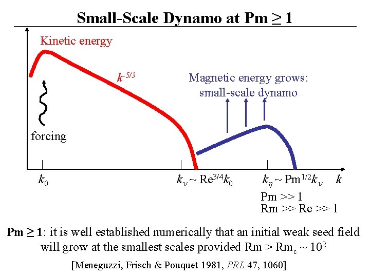
Small-Scale Dynamo at Pm ≥ 1 Kinetic energy k-5/3 Magnetic energy grows: small-scale dynamo forcing k 0 k ~ Re 3/4 k 0 k ~ Pm 1/2 k k Pm >> 1 Rm >> Re >> 1 Pm ≥ 1: it is well established numerically that an initial weak seed field will grow at the smallest scales provided Rm > Rmc ~ 102 [Meneguzzi, Frisch & Pouquet 1981, PRL 47, 1060]

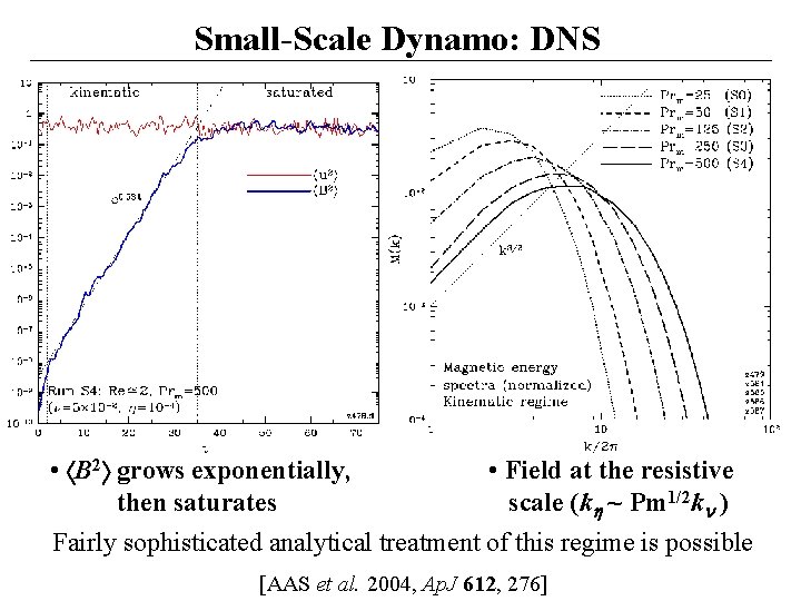
Small-Scale Dynamo: DNS • B 2 grows exponentially, • Field at the resistive then saturates scale (k ~ Pm 1/2 k ) Fairly sophisticated analytical treatment of this regime is possible [AAS et al. 2004, Ap. J 612, 276]

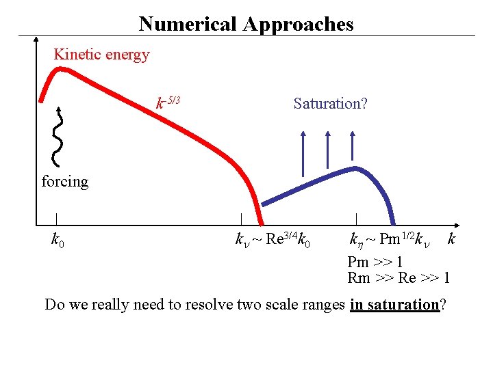
Numerical Approaches Kinetic energy k-5/3 Saturation? forcing k 0 k ~ Re 3/4 k 0 k ~ Pm 1/2 k k Pm >> 1 Rm >> Re >> 1 Do we really need to resolve two scale ranges in saturation?

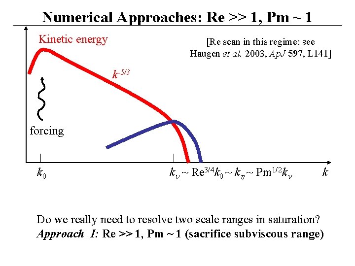
Numerical Approaches: Re >> 1, Pm ~ 1 Kinetic energy [Re scan in this regime: see Haugen et al. 2003, Ap. J 597, L 141] k-5/3 forcing k 0 k ~ Re 3/4 k 0 ~ k ~ Pm 1/2 k k Do we really need to resolve two scale ranges in saturation? Approach I: Re >> 1, Pm ~ 1 (sacrifice subviscous range)

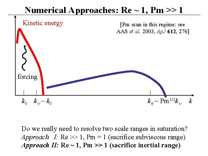
Numerical Approaches: Re ~ 1, Pm >> 1 Kinetic energy [Pm scan in this regime: see AAS et al. 2003, Ap. J 612, 276] forcing k 0 k ~ Pm 1/2 k Do we really need to resolve two scale ranges in saturation? Approach I: Re >> 1, Pm = 1 (sacrifice subviscous range) Approach II: Re ~ 1, Pm >> 1 (sacrifice inertial range) k

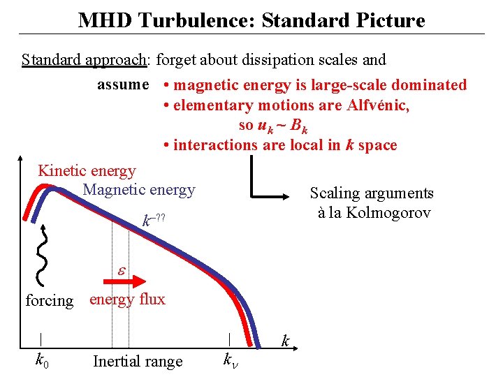
MHD Turbulence: Standard Picture Standard approach: forget about dissipation scales and assume • magnetic energy is large-scale dominated • elementary motions are Alfvénic, so uk ~ Bk • interactions are local in k space Kinetic energy Magnetic energy Scaling arguments à la Kolmogorov k–? ? forcing energy flux k 0 Inertial range k k

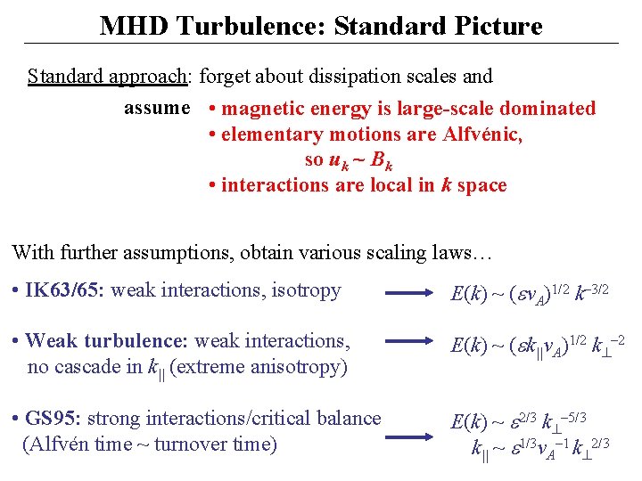
MHD Turbulence: Standard Picture Standard approach: forget about dissipation scales and assume • magnetic energy is large-scale dominated • elementary motions are Alfvénic, so uk ~ Bk • interactions are local in k space With further assumptions, obtain various scaling laws… • IK 63/65: weak interactions, isotropy E(k) ~ ( v. A)1/2 k– 3/2 • Weak turbulence: weak interactions, no cascade in k|| (extreme anisotropy) E(k) ~ ( k||v. A)1/2 k – 2 • GS 95: strong interactions/critical balance (Alfvén time ~ turnover time) E(k) ~ 2/3 k – 5/3 k|| ~ 1/3 v. A– 1 k 2/3

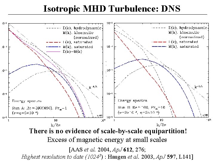
Isotropic MHD Turbulence: DNS There is no evidence of scale-by-scale equipartition! Excess of magnetic energy at small scales [AAS et al. 2004, Ap. J 612, 276; Highest resolution to date (10243) : Haugen et al. 2003, Ap. J 597, L 141]

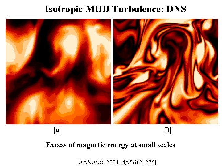
Isotropic MHD Turbulence: DNS |u| |B| Excess of magnetic energy at small scales [AAS et al. 2004, Ap. J 612, 276]

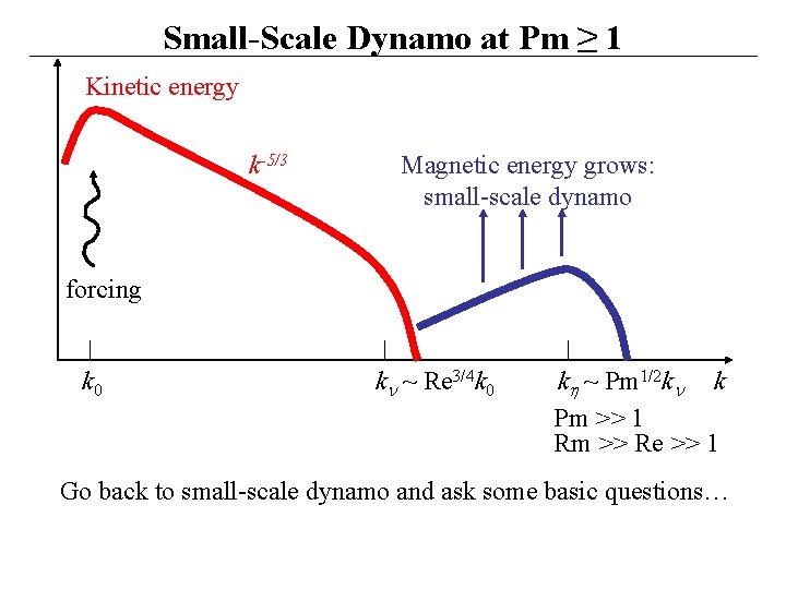
Small-Scale Dynamo at Pm ≥ 1 Kinetic energy k-5/3 Magnetic energy grows: small-scale dynamo forcing k 0 k ~ Re 3/4 k 0 k ~ Pm 1/2 k k Pm >> 1 Rm >> Re >> 1 Go back to small-scale dynamo and ask some basic questions…

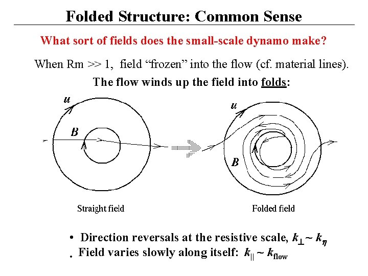
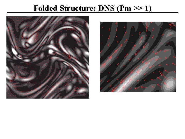
Folded Structure: Common Sense What sort of fields does the small-scale dynamo make? When Rm >> 1, field “frozen” into the flow (cf. material lines). The flow winds up the field into folds: • Direction reversals at the resistive scale, k ~ k • Field varies slowly along itself: k|| ~ kflow

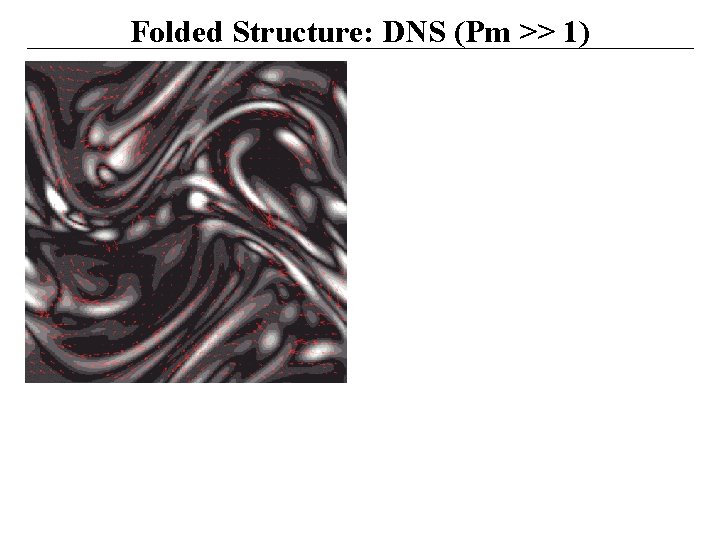
Folded Structure: DNS (Pm >> 1)

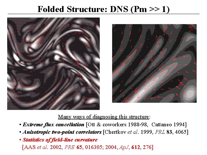
Folded Structure: DNS (Pm >> 1) Many ways of diagnosing this structure: • Extreme flux cancellation [Ott & coworkers 1988 -98, Cattaneo 1994] • Anisotropic two-point correlators [Chertkov et al. 1999, PRL 83, 4065] • Statistics of field-line curvature [AAS et al. 2002, PRE 65, 016305; 2004, Ap. J, 612, 276]

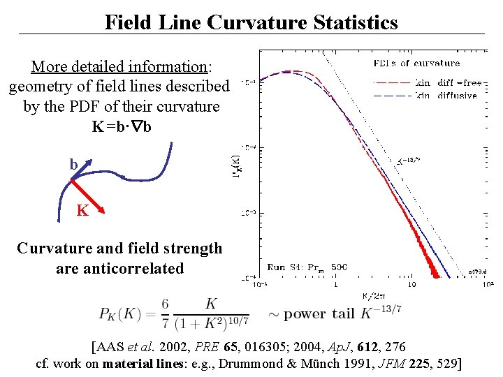
Field Line Curvature Statistics More detailed information: geometry of field lines described by the PDF of their curvature K=b· b b K Curvature and field strength are anticorrelated [AAS et al. 2002, PRE 65, 016305; 2004, Ap. J, 612, 276 cf. work on material lines: e. g. , Drummond & Münch 1991, JFM 225, 529]

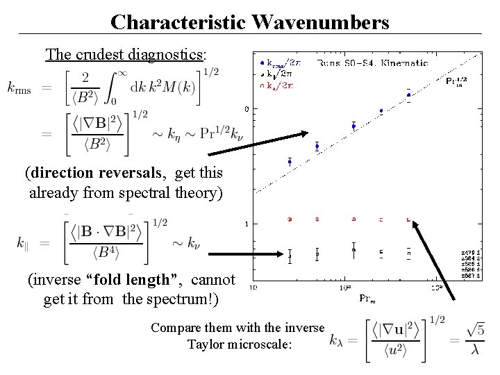
Characteristic Wavenumbers The crudest diagnostics: (direction reversals, get this already from spectral theory) (inverse “fold length”, cannot get it from the spectrum!) Compare them with the inverse Taylor microscale:

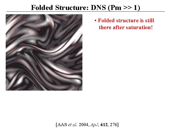
Folded Structure: DNS (Pm >> 1) • Folded structure is still there after saturation! [AAS et al. 2004, Ap. J, 612, 276]

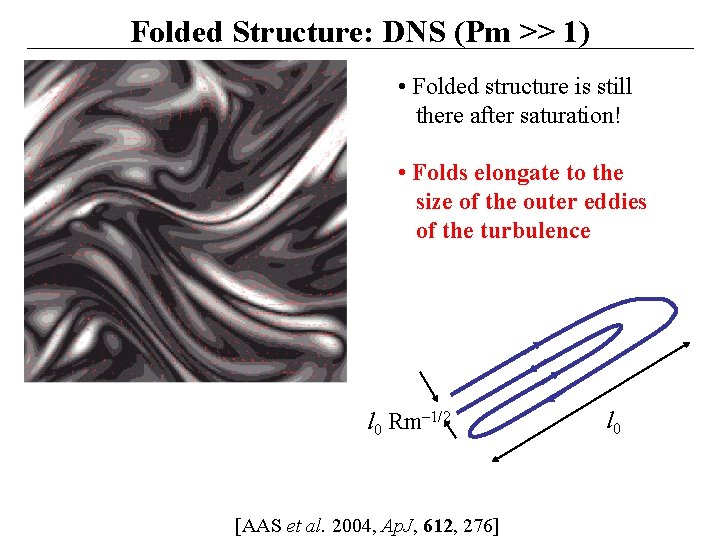
Folded Structure: DNS (Pm >> 1) • Folded structure is still there after saturation! • Folds elongate to the size of the outer eddies of the turbulence l 0 Rm– 1/2 [AAS et al. 2004, Ap. J, 612, 276] l 0

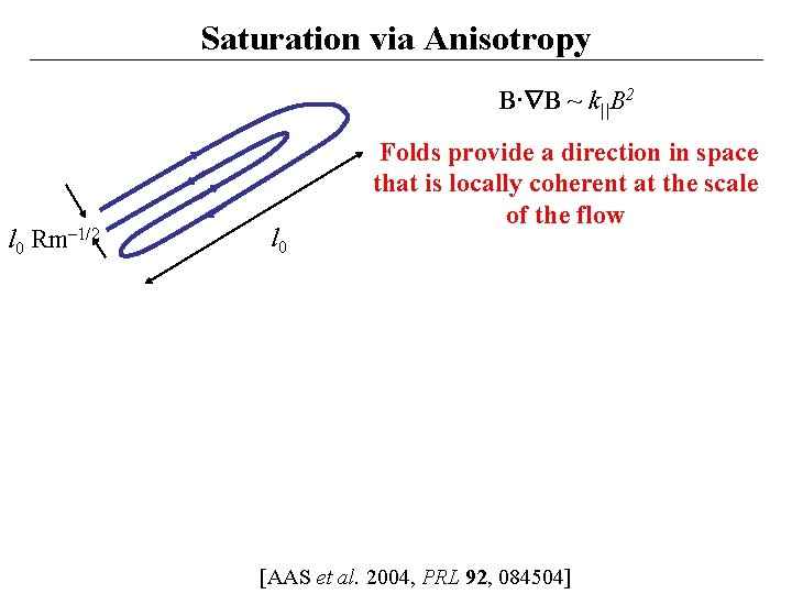
Saturation via Anisotropy B· B ~ k||B 2 l 0 Rm– 1/2 l 0 Folds provide a direction in space that is locally coherent at the scale of the flow [AAS et al. 2004, PRL 92, 084504]

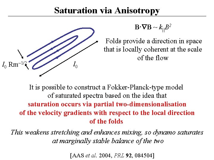
Saturation via Anisotropy B· B ~ k||B 2 l 0 Rm– 1/2 l 0 Folds provide a direction in space that is locally coherent at the scale of the flow It is possible to construct a Fokker-Planck-type model of saturated spectra based on the idea that saturation occurs via partial two-dimensionalisation of the velocity gradients with respect to the local direction of the folds This weakens stretching and enhances mixing, so dynamo saturates at marginally stable balance of the two [AAS et al. 2004, PRL 92, 084504]

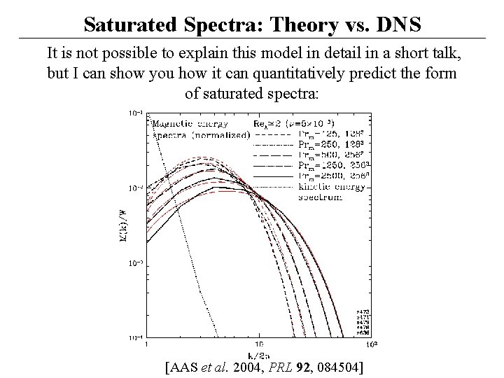
Saturated Spectra: Theory vs. DNS It is not possible to explain this model in detail in a short talk, but I can show you how it can quantitatively predict the form of saturated spectra: [AAS et al. 2004, PRL 92, 084504]

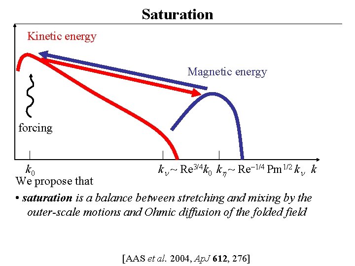
Saturation Kinetic energy Magnetic energy forcing k 0 k ~ Re 3/4 k 0 k ~ Re– 1/4 Pm 1/2 k k We propose that • saturation is a balance between stretching and mixing by the outer-scale motions and Ohmic diffusion of the folded field [AAS et al. 2004, Ap. J 612, 276]

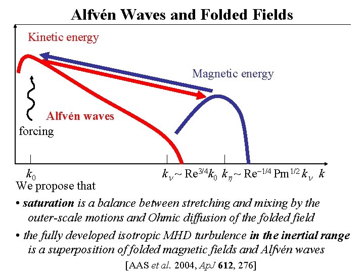
Alfvén Waves and Folded Fields Kinetic energy Magnetic energy Alfvén waves forcing k 0 k ~ Re 3/4 k 0 k ~ Re– 1/4 Pm 1/2 k k We propose that • saturation is a balance between stretching and mixing by the outer-scale motions and Ohmic diffusion of the folded field • the fully developed isotropic MHD turbulence in the inertial range is a superposition of folded magnetic fields and Alfvén waves [AAS et al. 2004, Ap. J 612, 276]

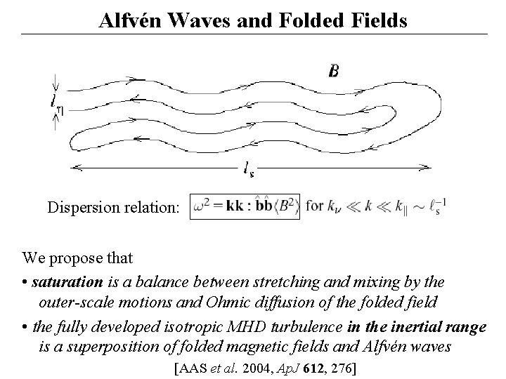
Alfvén Waves and Folded Fields Dispersion relation: We propose that • saturation is a balance between stretching and mixing by the outer-scale motions and Ohmic diffusion of the folded field • the fully developed isotropic MHD turbulence in the inertial range is a superposition of folded magnetic fields and Alfvén waves [AAS et al. 2004, Ap. J 612, 276]

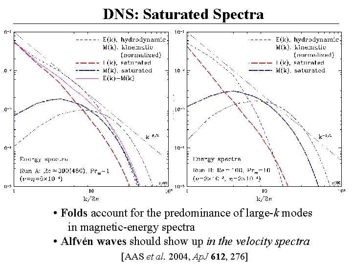
DNS: Saturated Spectra • Folds account for the predominance of large-k modes in magnetic-energy spectra • Alfvén waves should show up in the velocity spectra [AAS et al. 2004, Ap. J 612, 276]

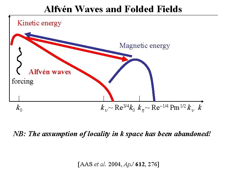
Alfvén Waves and Folded Fields Kinetic energy Magnetic energy Alfvén waves forcing k 0 k ~ Re 3/4 k 0 k ~ Re– 1/4 Pm 1/2 k k NB: The assumption of locality in k space has been abandoned! [AAS et al. 2004, Ap. J 612, 276]

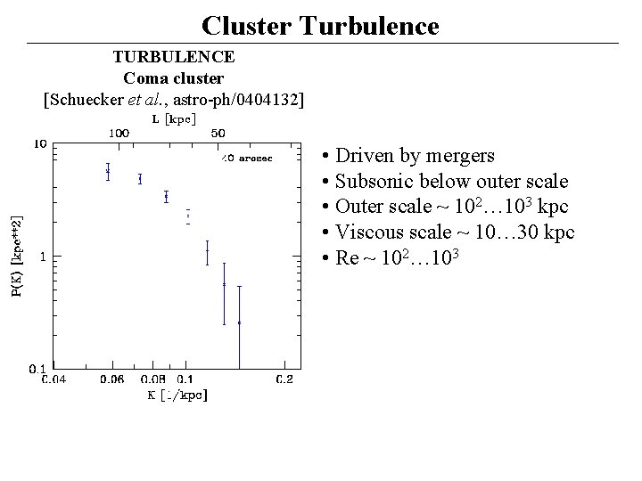
Cluster Turbulence TURBULENCE Coma cluster [Schuecker et al. , astro-ph/0404132] • Driven by mergers • Subsonic below outer scale • Outer scale ~ 102… 103 kpc • Viscous scale ~ 10… 30 kpc • Re ~ 102… 103

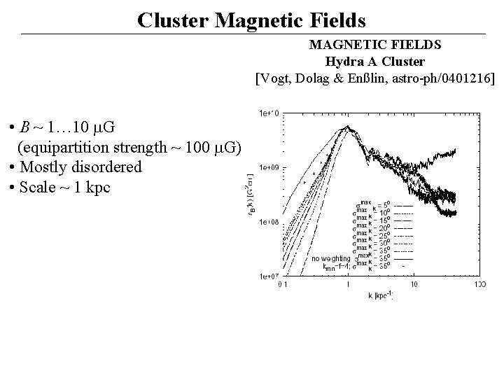
Cluster Magnetic Fields MAGNETIC FIELDS Hydra A Cluster [Vogt, Dolag & Enßlin, astro-ph/0401216] • B ~ 1… 10 G (equipartition strength ~ 100 G) • Mostly disordered • Scale ~ 1 kpc

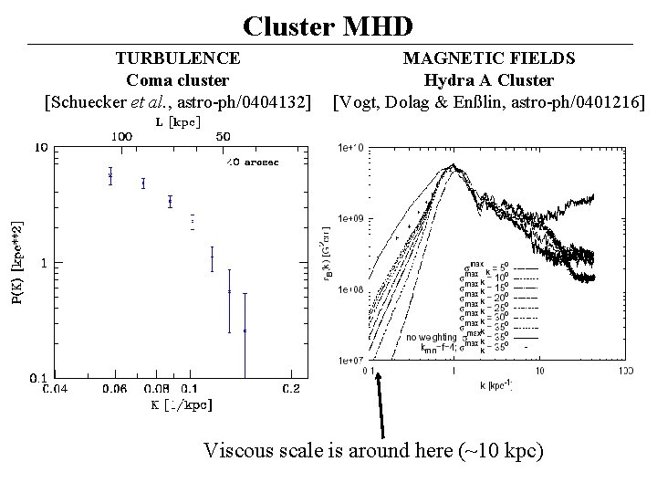
Cluster MHD TURBULENCE Coma cluster [Schuecker et al. , astro-ph/0404132] MAGNETIC FIELDS Hydra A Cluster [Vogt, Dolag & Enßlin, astro-ph/0401216] Viscous scale is around here (~10 kpc)

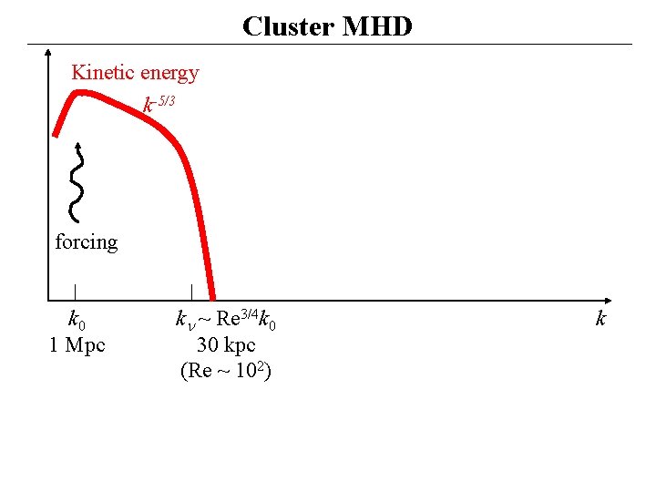
Cluster MHD Kinetic energy k-5/3 forcing k 0 1 Mpc k ~ Re 3/4 k 0 30 kpc (Re ~ 102) k

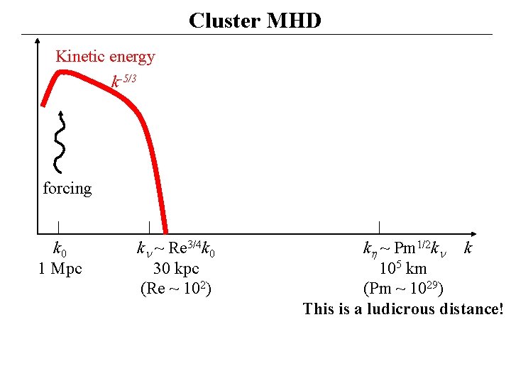
Cluster MHD Kinetic energy k-5/3 forcing k 0 1 Mpc k ~ Re 3/4 k 0 30 kpc (Re ~ 102) k ~ Pm 1/2 k k 105 km (Pm ~ 1029) This is a ludicrous distance!

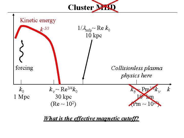
Cluster MHD Kinetic energy k-5/3 forcing k 0 1 Mpc 1/ mfp~ Re k 0 10 kpc Collisionless plasma physics here k ~ Re 3/4 k 0 30 kpc (Re ~ 102) k ~ Pm 1/2 k 105 km (Pm ~ 1029) What is the effective magnetic cutoff? k

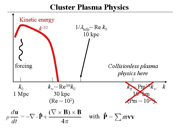
Cluster Plasma Physics Kinetic energy k-5/3 1/ mfp~ Re k 0 10 kpc forcing k 0 1 Mpc Collisionless plasma physics here k ~ Re 3/4 k 0 30 kpc (Re ~ 102) k ~ Pm 1/2 k 105 km (Pm ~ 1029) with k

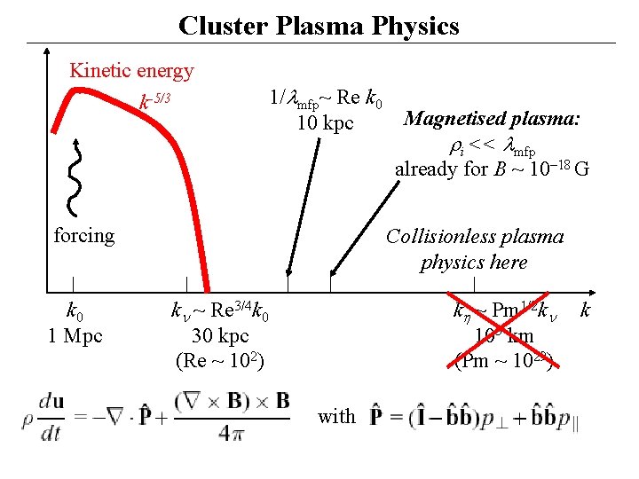
Cluster Plasma Physics Kinetic energy k-5/3 1/ mfp~ Re k 0 10 kpc forcing k 0 1 Mpc Magnetised plasma: i << mfp already for B ~ 10– 18 G Collisionless plasma physics here k ~ Re 3/4 k 0 30 kpc (Re ~ 102) k ~ Pm 1/2 k 105 km (Pm ~ 1029) with k

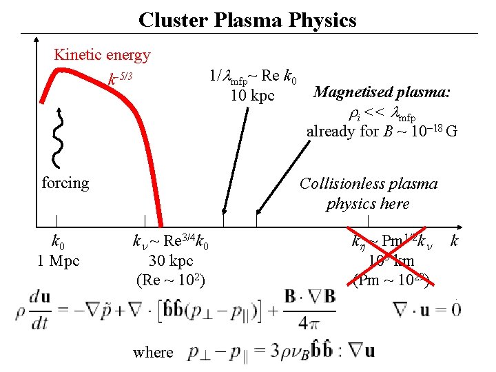
Cluster Plasma Physics Kinetic energy k-5/3 forcing k 0 1 Mpc 1/ mfp~ Re k 0 10 kpc Magnetised plasma: i << mfp already for B ~ 10– 18 G Collisionless plasma physics here k ~ Re 3/4 k 0 30 kpc (Re ~ 102) where k ~ Pm 1/2 k 105 km (Pm ~ 1029) k

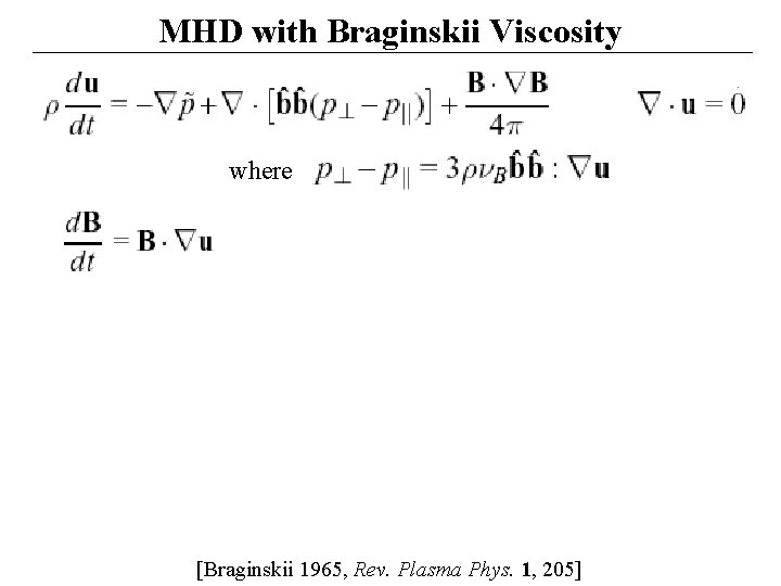
MHD with Braginskii Viscosity where [Braginskii 1965, Rev. Plasma Phys. 1, 205]

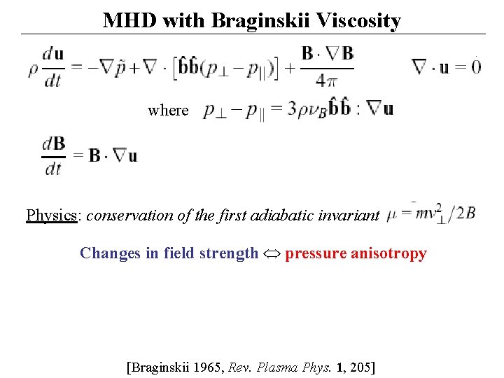
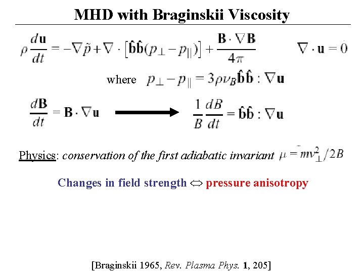
MHD with Braginskii Viscosity where Physics: conservation of the first adiabatic invariant Changes in field strength pressure anisotropy [Braginskii 1965, Rev. Plasma Phys. 1, 205]

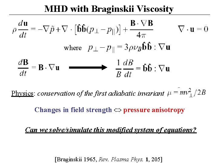
MHD with Braginskii Viscosity where Physics: conservation of the first adiabatic invariant Changes in field strength pressure anisotropy Can we solve/simulate this modified system of equations? [Braginskii 1965, Rev. Plasma Phys. 1, 205]

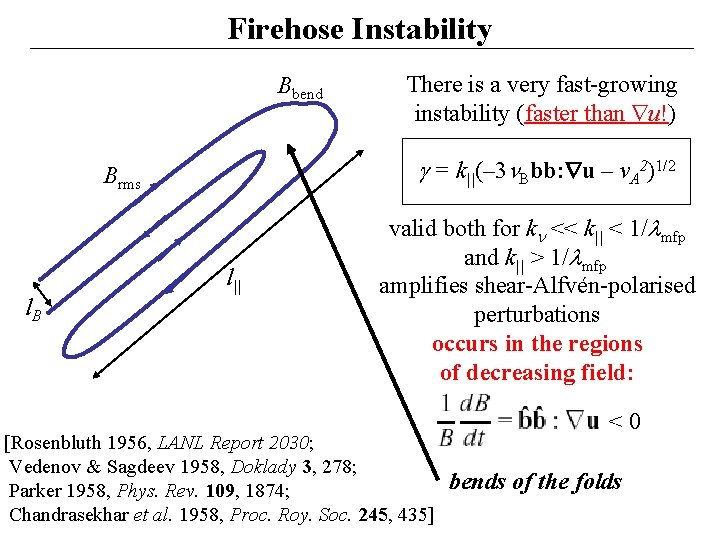
Firehose Instability Bbend = k||(– 3 Bbb: u – v. A 2)1/2 Brms l. B There is a very fast-growing instability (faster than u!) l|| valid both for k << k|| < 1/ mfp and k|| > 1/ mfp amplifies shear-Alfvén-polarised perturbations occurs in the regions of decreasing field: [Rosenbluth 1956, LANL Report 2030; Vedenov & Sagdeev 1958, Doklady 3, 278; Parker 1958, Phys. Rev. 109, 1874; Chandrasekhar et al. 1958, Proc. Roy. Soc. 245, 435] <0 bends of the folds

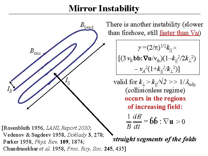
Mirror Instability Bbend There is another instability (slower than firehose, still faster than u) =(2/ )1/2 k|| Brms [(3 Bbb: u/vth)(1–k||2/2 k 2) – v. A 2(1+k||2/k 2)] l. B l|| valid for k > k||/√ 2 >> 1/ mfp (collisionless regime) occurs in the regions of increasing field: [Rosenbluth 1956, LANL Report 2030; Vedenov & Sagdeev 1958, Doklady 3, 278; straight segments Parker 1958, Phys. Rev. 109, 1874; Chandrasekhar et al. 1958, Proc. Roy. Soc. 245, 435] >0 of the folds

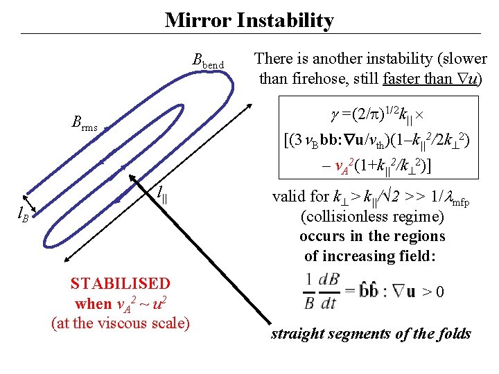
Mirror Instability Bbend There is another instability (slower than firehose, still faster than u) =(2/ )1/2 k|| Brms [(3 Bbb: u/vth)(1–k||2/2 k 2) – v. A 2(1+k||2/k 2)] l. B l|| STABILISED when v. A 2 ~ u 2 (at the viscous scale) valid for k > k||/√ 2 >> 1/ mfp (collisionless regime) occurs in the regions of increasing field: >0 straight segments of the folds

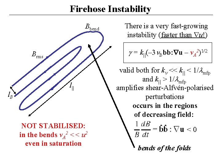
Firehose Instability Bbend = k||(– 3 Bbb: u – v. A 2)1/2 Brms l. B There is a very fast-growing instability (faster than u!) l|| NOT STABILISED: in the bends v. A 2 << u 2 even in saturation valid both for k << k|| < 1/ mfp and k|| > 1/ mfp amplifies shear-Alfvén-polarised perturbations occurs in the regions of decreasing field: <0 bends of the folds

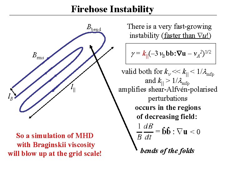
Firehose Instability Bbend = k||(– 3 Bbb: u – v. A 2)1/2 Brms l. B There is a very fast-growing instability (faster than u!) l|| So a simulation of MHD with Braginskii viscosity will blow up at the grid scale! valid both for k << k|| < 1/ mfp and k|| > 1/ mfp amplifies shear-Alfvén-polarised perturbations occurs in the regions of decreasing field: <0 bends of the folds

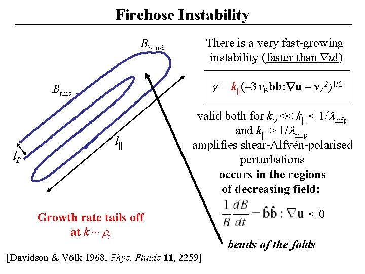
Firehose Instability There is a very fast-growing instability (faster than u!) Bbend = k||(– 3 Bbb: u – v. A 2)1/2 Brms l. B l|| valid both for k << k|| < 1/ mfp and k|| > 1/ mfp amplifies shear-Alfvén-polarised perturbations occurs in the regions of decreasing field: Growth rate tails off at k ~ i [Davidson & Völk 1968, Phys. Fluids 11, 2259] <0 bends of the folds

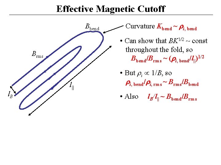
Effective Magnetic Cutoff Bbend • Can show that BK 1/2 ~ const throughout the fold, so Bbend/Brms ~ ( i, bend/l||)1/2 Brms l. B Curvature Kbend ~ i, bend l|| • But i 1/B, so i, bend/ i, rms ~ Brms/Bbend • Also l. B/l|| ~ Bbend/Brms

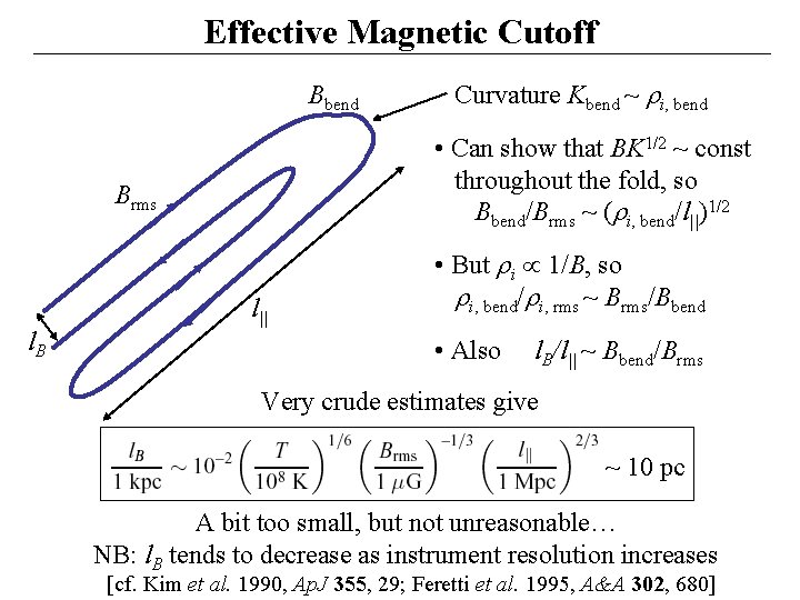
Effective Magnetic Cutoff Bbend • Can show that BK 1/2 ~ const throughout the fold, so Bbend/Brms ~ ( i, bend/l||)1/2 Brms l. B Curvature Kbend ~ i, bend l|| • But i 1/B, so i, bend/ i, rms ~ Brms/Bbend • Also l. B/l|| ~ Bbend/Brms Very crude estimates give ~ 10 pc A bit too small, but not unreasonable… NB: l. B tends to decrease as instrument resolution increases [cf. Kim et al. 1990, Ap. J 355, 29; Feretti et al. 1995, A&A 302, 680]

Poetry in Lieu of Summary James Clerk Maxwell on the inevitability of kinetic description of cluster plasmas At quite uncertain times and places, The atoms left their heavenly path, And by fortuitous embraces, Engendered all that being hath. And though they seem to cling together, And form “associations” here, Yet, soon or late, they burst their tether, And through the depths of space career. 1874