Tugas Pengukran dan Instrumentasi Kelompok 10 Maulana Ishaq
 Novan Ady")

(iw) for everything following the demodolator should be K < 0 o")


, the following")


 (the actual measured data) is known")
 = Qi(iῶ) �Di Inverskan : Qi(iῶ) =")
 whether the measurement system meets the")


 of first-order dynamic character-istics is avaliable from")


 then would be the actual input (qi) to the measuring device,")
 velocity")
, and thus admittance is the")


- Slides: 28
Tugas Pengukran dan Instrumentasi Kelompok 10 : Maulana Ishaq F. S (145060209111002) Novan Ady Sasongko (145060209111003) Muhamad ‘Ainul Yaqin (145060209111004)
Requirements on Instument Transfer Function to Ensure Accurate Measurement � 1. For perfect shape reproduction with no time delay between (qi) and (qo) and with : �Periodict inputs (qo/qi)(iῶ) must equal K < 0 o for all frequencies contained in qi with significant amplitude. �Transient inputs (qo/qi) (iw) must equal K < 0 o for the entire frequency range in which the fourier transform of qi(t) has significant magnitude. �Amplitude-modulated signals. Same criteria as in parts a and b, depending on whether the modulating signal is periodic or transient.
�Demodulated signals. (qo/qi)(iw) for everything following the demodolator should be K < 0 o for all significant frequency bands of the modulating signal and should be zero for all carrier and side frequency bands producced by the modulating process. �Random signals (qo/qi)(iw) must equal K< 0 o over the entire frequency band where ᶲqi (w) is significantly larger to zero.
�While popur choice of parameters allows many measurement systems to meet the requirement of flat amplitudo ratio, the simultaneous achievement of near-zero phase angle over the same frequency range is rarely possible (second order instruments with small ζ and large ῶn, such as piezoelectric devices, are an exception).
�This requirement results in qo being a perfect reproduction of qi however qo will be delayed in time by a spesific amount , as if the system contained a dead-time effect τdt. For many applications , the fact that q 0 appers on our oscilloscope screen or recorder chart τdt seconds “late” is of no importance whatever. Thus requiring a system frequency respons of K < (ῶτdt) is widely acceptable. There are, however two situations in which such time (phase) shift might cause difficulty.
�In multichannel systems, unless each channel has the same τdt (not likely), the following happens if you pick, say a gas-temperature value form channel 1 and gas-pressure value form channel 4, by using the same chart-paper time value, any computed gas density value would be wrong because the temperature and pressure values, while aligned on the chart , were not simultaneous in actual time occurrence.
�Of course, if you know the τdt values for each channel, suitable corrections can be applied, perhaps including those in a computer program used for data reduction. In fact, by using microprocessor tecnology, these corrections could be made part of the multichannel recorder itself, with each channel being properly shifted in time befor it is written on the chart. The second type of application where K < (-ῶτdt) suffers relative to K < 0 o occurs when the measuring system is embedded in a feedback control loop. Here phase lag detracts from system stability and should be minimized.
Revising our earlier accuracy statement, we now say: � 2. For perfect shape reproduction with time delay τdt between qi and qo and with: �Periodic inputs �Transient �Amplitudo-moulated signals �Demodulated signals �Random signals �Same as 1 except that wherever (qo/qi)(iῶ)=K<0 o is required. Now (qo/qi)(iῶ)=K< (-ῶτdt) is required. That is amplitude ratio constant but phase lag increases linerly with frequency ῶ.
Numerical Correction of Dynamic Data Theoretically, if qo(t) (the actual measured data) is known and if (qo/qi)(iῶ) for the measurement system is known, we can always reconstruct a perfect record of qi(t) by the following process: �Transform qo(t) to Qo(iῶ) �Apply the formula
�Qo(iῶ) = Qi(iῶ) �Di Inverskan : Qi(iῶ) =
�This prosedure theoretically will give the exact qi(t) whether the measurement system meets the K < (-ῶτdt) requirement or not. In actual practice, of coure, while the measurement system does not have to meet K < (-ῶτdt) , it does have to respond fairly strongly to all frequencies present in qi ; otherwise, some parts of the qo frequency spectrum will be so small as to be submerged in the unavioidable “noise” present in all systems and thus be unreconverable by the above mathematical process. As general-purpose digital computers are used more in data prosessing and as computing power is built into more “instrument” such dynamic correction becomes increasingly practical and is a usable alternative in those situations where measurement systems meeting K < (ῶτdt) cannot be constructed with the present state of the art. Many FFT signal /system analyzers have this capability built into their software.
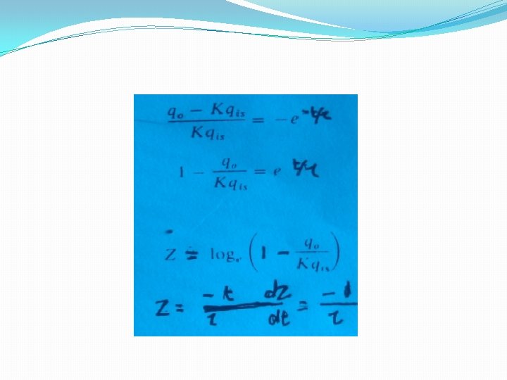
Experimental Determination of Measurement. System Parameters �While theoritical analysis of instrument is vital to reveal the basic relationships involved in the operation device, it is rarely accurate enaugh to provide usable numerical values for critical parameters such as sensitivity, time constan, natural frequency, etc. The only parameter to be determined is the static sensitivity K, which is found by static calibration. For first-order instrument, the static sensitivity K also is found by static calibration. this method influenced by inaccuracies in the determination of the t=0 point and also gives no check as to whether the instrument is really first-order. This methode goes as follows : from 3. 143 we can write
�Thus if we plot z versus t, we get a straight line whose slope is numerically. This gives a more accurate value of since the best line through all the data poinst is used rather than just two points, as in the 63. 2 percent methode. Figure 3. 99 illustrastes the procedure
� An even stronger verivication (or refutation) of first-order dynamic character-istics is avaliable from frequency-response testing, although at considerable cost of time and money if the system is not completely electrical, since nonelectrical sinewave generators are neither common nor necessarily cheap. If the system is truly first-order, the amplitude ratio follows the typical low and high frequency asymptotes ( slope 0 and 20 db/decade) and the phase angel approaches-90 asymptotically. If these characteristics are present, the numerical value of τ is found by determining w at the breakpoint and using τ =1/w break (seefigure 3. 100). deviations from the above amplitude and/or phase characteristics indicate non-first-order behavior.
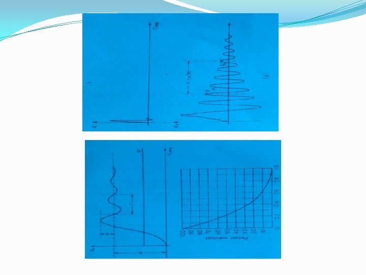
�For second-order systems, K is found from static calibration, and ζ and ωn can be obtained in a number of ways from step or frequency-response test. Figure 3. 101 a shows a typical step-fuction response for an underdamped second-order system. The values of ζ and ωn may be found from the relations. When a system is lightly damped, any fast transient input will produce a response similar to fig. 3. 101 b. then ζ can be closely approximated by
If a system is strictly linear and second-order, the value of n in Eq. (3. 321) is immaterial ; the same value of x will be found for any number of cycles. Thus if ζ is calculated for, say, n= 1, 2, 4, and 6 and different numerical values of x are obtained, we know the system is not following the posttulated mathematical model. From eq ( 3. 202 ) we can write
To find ζ 1 and ζ 2 from a step fuction- response curve, we may proceed as follows : 1. Define the percent incomplete response Rpi as 2. Plot Rpi on a logarithmic scale versus time t on a linear scale. This curve will approach a straight line for large t if the system is second-order. Extend this line back to t =0, and note value P 1 where this line intersects the Rpi scale. Now , ζ 1 is the time at which the straight-line asymptote has the value 0, 368 P 1. Now plot on the same graph a new curve which is the 3. difference between the straight-line asymptote and Rpi. If this new curve is not a straight line, the system is not second-order. If it is a straight line, the time at which this line has the value 0, 368(p 1 -100) is numerically equal to ζ 2
Figure 3. 102 ilustrates this produce. once τ1 and τ2 are found , ζ and ωn can be determined from eqs(3. 323) and (3. 324) if desired. Other methods 2 for finding τ1 and τ2 are available in the literature. Frequency – response methods also may be used to find ζ and ωn or τ1 and τ2
Loading Effects under Dynamic Conditions �The treatment of loading effects by means of impedance, admittance, etc. All these results can immediately transferred to the case of dynamic operation by generalizing the definitions in term of transfer function. The basic equations are :
�The quantities Z, Y, S and C previously were considered to be the ratios of small changes in two related system variables under stated conditions. �Usually the frequency response form is most useful if these quantities must be found experimentally. �This causes a sinusoidal change in the other ("output") variable, and thus we can speak of an amplitude ratio and phase angle between these two quantities, making Z(iω) now a complex number that varies with frequency.
�The quantity (qilm) then would be the actual input (qi) to the measuring device, and we could calculate (qo) if the transfer function (qo/qi)(iω) were known. that is, Thus we could define a loaded transfer function (qo/qi)(iω) as where qo * actual output of measuring device that has no load at its output qwu * measured variable value that would exist if measuring device cause no loading on measured medium
�The unloaded transfer function relating the output displacement xo and the input (measured) velocity vi is obtained as follows : Where (Ki) * instrument static sensitivity
�since the measured quantity is velocity (a flow variable), and thus admittance is the appropriate quantity to use. We determine the input admittance (Ygi(D))=(v/f)(D) from Fig. 3. 104 c as follows: �Also �and, eliminating (xo), we get
Figure 3. 104 Example of dynamic loading analysis.
�Consider a device for measuring translational velocity, as in fig. 3. 104 a. �Suppose we now attach this instrument to a vibrating system whose velocity we wish to measure, as in fig. 3. 104 b. �The character of this distortion may be assessed by aplication or Eq. (3. 61), since the measured quantity is velocity (a flow variable), and thus admittance is the appropriate quantity to use. We determine the input admittance (Ygi(D))=(v/f)(D) from Fig. 3. 104 c as follows:
�Figure 3. 104 c also shows the frequency characteristics of this input admittanc. The output admittance (Ygo)=(v/f)(D) of the measured system is obtained from Fig. 3. 104 d: �Figure 3. 104 e shows that in this example the loading efect is most serious for frequencies near the natural frequency of the measured system, but approaches zero for both very low and very high frequencies. Since the loading effects can be expressed in frequency terms, they can be handled for all kinds of inputs by using appropriate Fourier series, transform, or mean square spectral density.