Tuesday October 1 Point Estimation Using SPSS and
Tuesday October 1 Point Estimation; Using SPSS and Excel to conduct ttests
Last Time • We practiced doing an independent samples ttest by hand • We learned how to do related samples t-tests – We learned when to do this type of test (one group, two scores person, or two groups with pairs of participants who are matched or related in some way – We learned that this test is essentially the same as a one-sample t-test on difference scores, with H 0: μD=0 – We learned how to do a related samples t-test in SPSS
Estimation • In inferential statistics we use sample statistics to make inferences about population parameters • One way we can do this is to estimate population parameters based on sample statistics • Estimate can be – Point estimate – Interval estimate – Confidence interval
Point Estimation – Single value (e. g. M is the point estimate of μ, or s is the estimate of σ) – Single value that represents a difference (e. g. , MD is the point estimate of μD, MA-MB is the point estimate of μA-μB) – Point estimates we are interested in are often in the numerators of our test statistics.
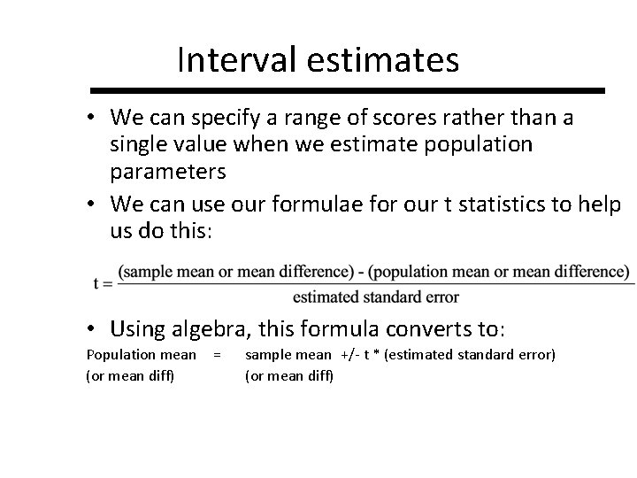
Interval estimates • We can specify a range of scores rather than a single value when we estimate population parameters • We can use our formulae for our t statistics to help us do this: • Using algebra, this formula converts to: Population mean (or mean diff) = sample mean +/- t * (estimated standard error) (or mean diff)
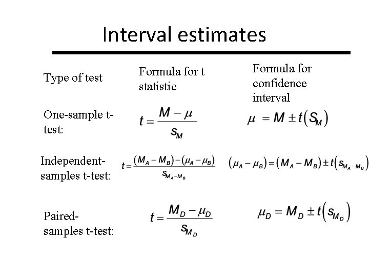
Interval estimates Type of test One-sample ttest: Independentsamples t-test: Pairedsamples t-test: Formula for t statistic Formula for confidence interval
Confidence Intervals • Interval estimate accompanied by specific level of confidence or probability (e. g. , p=. 95)
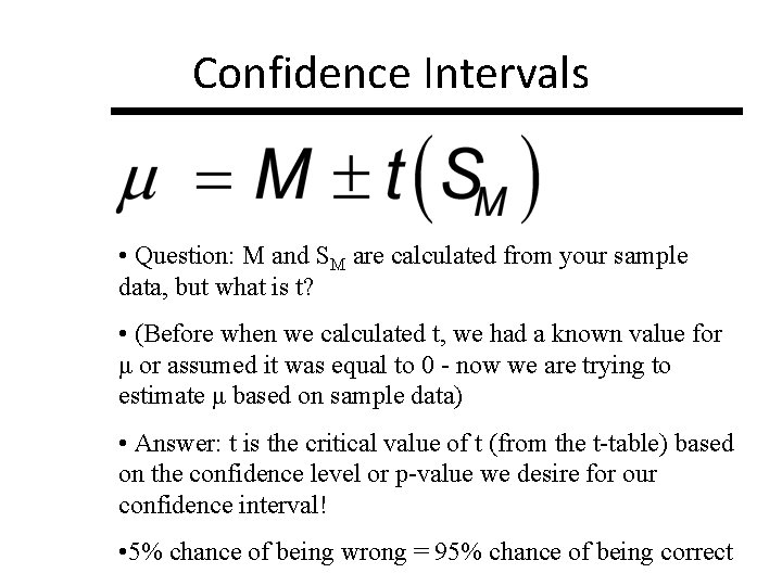
Confidence Intervals • Question: M and SM are calculated from your sample data, but what is t? • (Before when we calculated t, we had a known value for μ or assumed it was equal to 0 - now we are trying to estimate μ based on sample data) • Answer: t is the critical value of t (from the t-table) based on the confidence level or p-value we desire for our confidence interval! • 5% chance of being wrong = 95% chance of being correct
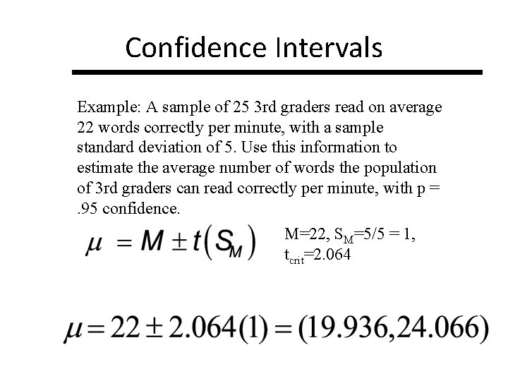
Confidence Intervals Example: A sample of 25 3 rd graders read on average 22 words correctly per minute, with a sample standard deviation of 5. Use this information to estimate the average number of words the population of 3 rd graders can read correctly per minute, with p =. 95 confidence. M=22, SM=5/5 = 1, tcrit=2. 064
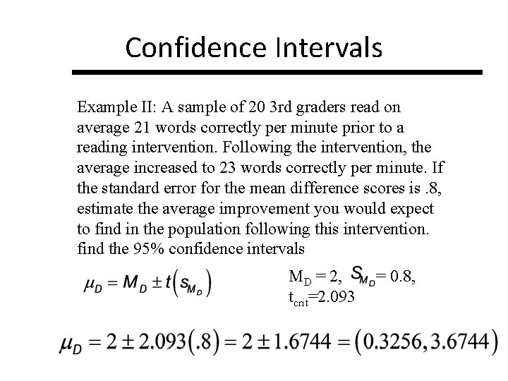
Confidence Intervals Example II: A sample of 20 3 rd graders read on average 21 words correctly per minute prior to a reading intervention. Following the intervention, the average increased to 23 words correctly per minute. If the standard error for the mean difference scores is. 8, estimate the average improvement you would expect to find in the population following this intervention. find the 95% confidence intervals MD = 2, tcrit=2. 093 = 0. 8,
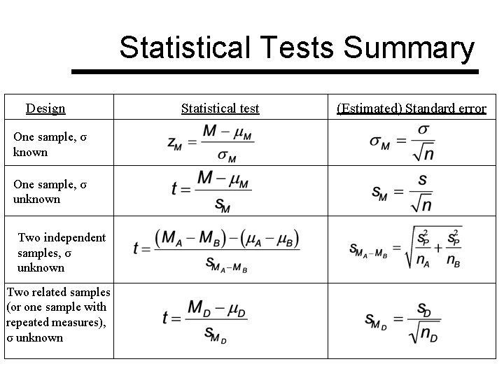
Statistical Tests Summary Design One sample, σ known One sample, σ unknown Two independent samples, σ unknown Two related samples (or one sample with repeated measures), σ unknown Statistical test (Estimated) Standard error
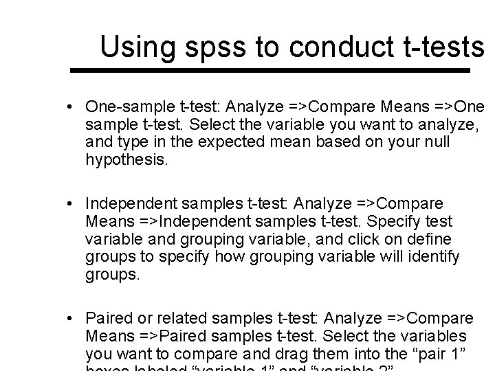
Using spss to conduct t-tests • One-sample t-test: Analyze =>Compare Means =>One sample t-test. Select the variable you want to analyze, and type in the expected mean based on your null hypothesis. • Independent samples t-test: Analyze =>Compare Means =>Independent samples t-test. Specify test variable and grouping variable, and click on define groups to specify how grouping variable will identify groups. • Paired or related samples t-test: Analyze =>Compare Means =>Paired samples t-test. Select the variables you want to compare and drag them into the “pair 1”
Using excel to compute ttests • =ttest(array 1, array 2, tails, type) • Select the arrays that you want to compare, specify number of tails (1 or 2) and type of t-test (1=dependent, 2=independent w/equal variance assumed, 3=independent w/unequal variance assumed). • Returns the p-value associated with the t-test.
Next Homework (due Thursday, October 3) See Handout
- Slides: 14