TS 4273 Traffic Engineering SIGNALISED INTERSECTIONS First Traffic

TS 4273 Traffic Engineering SIGNALISED INTERSECTIONS

First Traffic Light • Traffic lights were used before the advent of the motorcar. In 1868, British railroad signal engineer J P Knight invented the first traffic light, a lantern with red and green signals. • It was installed at the intersection of George and Bridge Streets in front of the British House of Commons to control the flow of horse buggies and pedestrians. http: //www. didyouknow. cd/trafficlights. htm

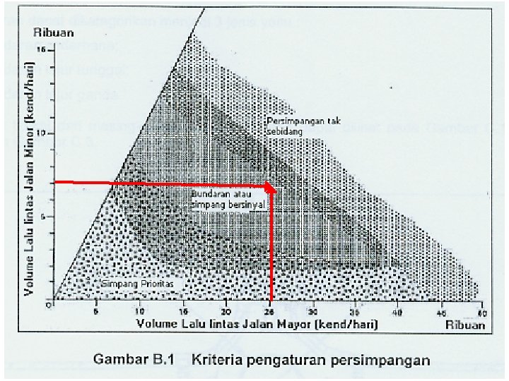
Prinsip-prinsip desain simpang bersinyal • Suatu persimpangan membutuhkan lampu lalulintas jika waktu tunggu rata-rata kendaraan sudah lebih besar daripada waktu tunggu rata-rata kendaraan pada persimpangan dengan lampu lalulintas.

Prinsip-prinsip desain simpang bersinyal Waktu tunggu rata-rata kendaraan pada persimpangan bersinyal dipengaruhi oleh: • Arus lalulintas pada masing-masing arah, • Waktu antara kedatangan kendaraan dari masing-masing arah, • Keberanian pengemudi untuk menerima waktu antara yang tersedia guna menyeberangi jalan.

Prinsip-prinsip desain simpang bersinyal Delay Unsignalised Traffic Flow Signalised

Scope of IHCM Signalised Intersection Analyses • Isolated, fixed-time controlled signalised intersections with normal geometry layout (fourarm and three-arm) and traffic signal control devices. • Coordinated traffic signal control is normally needed if the distance to adjacent signalised intersections is small (< 200 m). Persimpangan Raya Darmo – Polisi Istimewa & Raya Darmo – RA Kartini.

Objectives of IHCM Signalised Intersection Analyses • To avoid blockage of an intersection by conflicting traffic streams, thus guaranteeing that a certain capacity can be maintained even during peak traffic conditions;

Objectives of IHCM Signalised Intersection Analyses • To facilitate the crossing of a major road by vehicles and/or pedestrians from a minor road; • To reduce the number of traffic accidents caused by collisions between vehicles in conflicting directions.

Potential Conflict at Intersections

Primary and Secondary Conflictis in a Four-Arm Signalised Intersections

Time Sequence for Two-Phase Signal Control Street A Street B

Time Sequence for Four-Phase Signal Control

Time Sequence for Two-Phase Signal Control Street A Street B

Purpose of the Intergreen Period • Warn discharging traffic that the phase is terminated. Amber Period (for urban traffic signal in Indonesia is normally 3, 0 sec) • Certify that the last vehicle in the green phase which is being terminated receives adequate time to evacuate the conflict zone before the first advancing vehicle in the next phase enters the same area. All-Red Period

Signal Phasing Arrangements • Introducing more than two phases normally leads to an increase of the cycle time and of the ratio of time allocated to switching between phases (especially for isolated and fixedcontrolled).

Signal Phasing Arrangements • Although this may be beneficial from the traffic safety point of view, it normally means that the overall capacity of the intersection is decreased.

Basic Model for Saturation Flow (Akcelik 1989)

Basic Model Saturation Flow • Discharge rate starts from 0 at the beginning of green and reaches its peak value after 10 -15 sec • Effective Green = Displayed Green Time – Start Loss + End Gain • Start loss End gain 4, 8 sec (MKJI p. 2 -12) • Effective Green = Displayed Green Time

Basic Model Saturation Flow • Base saturation flow is different between Protected approach and Opposed approach • For protected approach S 0 = 600 x We • For opposed approach S 0 in Indonesia usually lower where there is a high ratio of right turning movements, compare with Western models.

Perhitungan Arus Jenuh Metode Time Slice Arus jenuh/jam (3. 600/5)x 4, 5 = 3. 240 smp/jam Jika lebar lajur = 4, 0 m (3. 240/4) = 810 smp/jam/m Maka S = 810 x We

Traffic Safety Considerations • Traffic accident rate for signalised intersections has been estimated as 0, 43 accidents/million incoming vehicles as compare to 0, 60 for unsignalised intersections and 0, 30 for roundabouts.

STEP A-1: Geometric, Traffic Control and Environmental Conditions • • • General information (date, handled by, city, etc. ) City size (to the nearest 0, 1 M inhabitants) Signal phasing & timing Left turn on red (LTOR) Approach code Road environment and level of side friction Median Gradient Approach width (to the nearest tenth of a meter)

Geometry of Signalised Intersection

STEP A-2: Traffic Flow Conditions pce for Approach Type Vehicle Type Protected Opposed Light Vehicle (LV) 1, 0 Heavy Vehicle (HV) 1, 3 Motorcycle (MC) 0, 2 0, 4 Q = QLV + (QHV x pce. HV) + (QMC x pce. MC)

STEP B-1: Signal Phasing and Timing • If the number and types of signal phases are not known, two-phase control should be used as a base case. • Separate control of right-turning movements should normally only be considered if a turning-movement exceeds 200 pcu/h and has a separate lane.

STEP B-1: Signal Phasing and Timing • Early start = leading green one approach is given a short period before the start of the green also in the opposing direction (usually 25%-33% from total green time) • Late cut-off = lagging green the green light in one approach is extended a short period after the end of green in the opposing direction. • The length of the leading and the lagging green should not be shorter than 10 sec.

STEP B-2: Intergreen time and lost time Intersection Size Mean Road Width Intergreen Time Default Values Small 6– 9 m 4 sec/phase Medium 10 – 14 m 5 sec/phase Large ≥ 15 m ≥ 6 sec/phase Only for planning purposes !!!

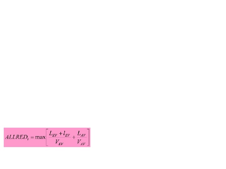
STEP B-2: Intergreen time and lost time For operational and design analysis !!! • LEV, LAV distance from stop line to conflict point for evacuating and advancing vehicle (m) • l. EV length of evacuating vehicle (m) • VEV, VAV speed of evacuating and advancing vehicle (m/sec)

STEP B-2: Intergreen time and lost time • • • VAV 10 m/sec (motor vehicles) VEV 3 m/sec (un-motorised) VEV 1, 2 m/sec (pedestrians) l. EV 5 m (LV or HV) l. EV 2 m (MC or UM)

STEP B-2: Intergreen time and lost time • IG Intergreen = Allred + Amber • The length of AMBER usually 3, 0 sec

STEP C-1: Approach Type PROTECTED (P) Discharge without any conflict between rightturning movements and straight-through/leftturning movements.

STEP C-1: Approach Type • OPPOSED (O) Discharge with conflict between right-turning movements and straightthrough/left-turning movements from different approaches with green in the same phase.

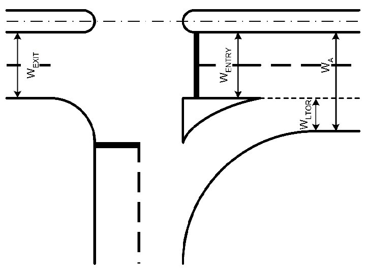
STEP C-2: Effective Aproach Width (We) Without LTOR • For Approach Type P (Q = QST) • If WEXIT We x (1 - p. RT - p. LT) We = WEXIT

STEP C-2: Effective Aproach Width (We) • If WLTOR ≥ 2 m (it is assumed that the LTOR vehicle can bypass the other vehicle) We = min { (WA-WLTOR) , (WENTRY) } • For Approach Type P (Q = QST) If WEXIT < We x (1 – p. RT) We = WEXIT

STEP C-2: Effective Aproach Width (We) • If WLTOR < 2 m (it is assumed that the LTOR vehicle cannot bypass the other vehicle) We = min { (WA) , (WENTRY+WLTOR) , (Wax(1+p. LTOR)-WLTOR) } • For Approach Type P (Q = QST) If WEXIT < We x (1 – p. RT – p. LTOR) We = WEXIT

STEP C-3: Base Saturation Flow (S) • For protected approach

STEP C-3: Base Saturation Flow (S) • For Approach Type P • S 0 base saturation flow (pcu/hg) • We effective width (m) • Figure C-3: 1 page 2 -49

STEP C-3: Base Saturation Flow (S) • For Approach Type O (opposed) • QRT and QRTO (Column 14 Form SIG-II opposed discharge right-turning) • Figure C-3: 2 page 2 -51 for approaches without separate right-turning. • Figure C-3: 3 page 2 -52 for approaches with separate right-turning. • Use interpolation if approach width larger or smaller than actual We

STEP C-3: Base Saturation Flow (S) • Ex: without separate right-turning lane QRT = 125 pcu/h, QRTO = 100 pcu/h Actual We = 5, 4 m Obtain from Figure C-3: 2 p. 2 -51 (We=5 & We=6) S 6, 0 = 3. 000 (pcu/hg) ; S 5, 0 = 2. 440 (pcu/hg) Calculate; S 5, 4 =(5, 4 -5, 0)x(S 6, 0 - S 5, 0)+ S 5, 0 =0, 4(3. 000 -2. 440)+2. 440 2. 660 (pcu/hg)

STEP C-3: Base Saturation Flow (S) • If right-turning movement > 250 pcu/h, protected signal phasing should be considered • For No Separate RT-lane • If QRTO < 250 pcu/h • Determine SPROV for QRTO = 250 pcu/h • Determine Actual S as • S = SPROV – [(QRTO - 250) x 8]pcu/h

STEP C-3: Base Saturation Flow (S) • • • For No Separate RT-lane If QRTO > 250 pcu/h Determine SPROV for QRTO and QRT= 250 pcu/h Determine Actual S as S = SPROV – [(QRTO + QRT - 500) x 2]pcu/h • If QRTO < 250 pcu/h and QRT > 250 pcu/h • Determine S as for QRT = 250 pcu/h

STEP C-3: Base Saturation Flow (S) • For Separate RT-lane • If QRTO > 250 pcu/h • QRT < 250 pcu/h Determine S from Figure C 3: 3 through extrapolation • QRT > 250 pcu/h Determine SPROV as for QRTO and QRT= 250 pcu/h • If QRTO < 250 pcu/h and QRT > 250 pcu/h • Determine S from Figure C 3: 3 through extrapolation

STEP C-4: City Size Adjustment Factor FCS [ Table C-4: 3 p. 2 -53] City Size Inhab. (M) FCS Very Small 0, 1 0, 82 Small > 0, 1 - 0, 5 0, 88 Medium > 0, 5 - 1, 0 0, 94 Large > 1, 0 - 3, 0 1, 00 Very Large > 3, 0 1, 05

STEP C-4: Side Friction Adjustment Factor FSF [ Table C-4: 4 p. 2 -53]

STEP C-4: Side Friction Adjustment Factor FSF [ Table C-4: 4 p. 2 -53]

STEP C-4: Side Friction Adjustment Factor FSF [ Table C-4: 4 p. 2 -53]

STEP C-4: Gradient Adjustments Factors FG [Figure C-4: 1 p. 2 -54] If G 0 1 – (0, 01 x G) If G < 0 1 – (0, 005 x G)

STEP C-4: Effect of Parking Adjustments Factors FP [Figure C-4: 2 p. 2 -54 • LP distance between stop-line and first parked vehicle (m) • WA Width of the approach (m) • g Green time in the approach (default value 26 sec) • It should not be applied in cases were the effective width is determined by the exit width.

STEP C-4: Right Turn Adjustments Factors FRT = 1. 0 + p. RT x 0. 26

STEP C-4: Left Turn Adjustments Factors FLT = 1. 0 - p. LT x 0. 16

Calculated the adjusted value of saturation flow S • • SO Base saturation flow FCS City size FSF Side friction FG Gradient FP Parking FRT Right turn FLT Left turn

STEP C-5: Flow/Saturation Flow Ratio • Calculate the Flow Ratio (FR) for each approach • Calculate the Intersection Flow Ratio (IFR) Sum of the critical (highest) flow ratios for all consecutive signal phases in a cycle • Calculate the Phase Ratio (PR) for each phase

STEP C-6: Cycle Time and Green Time • Unadjusted cycle time (Cua) LTI = S off all intergreen periods 2 phase 40 -80 sec 3 phase 50 -100 sec • Green time (g) 4 phase 80 -130 sec green times < 10 sec should be avoided !!! • Adjusted cycle time (c)

STEP D-1: Capacity • Calculate the capacity of each approach • Calculate the Degree of Saturation Acceptable value normally 0, 75 !!! If the signal timing has been correctly done, DS will be nearly the same in all critical approaches !!!

STEP D-2: Need For Revisions • Increase of approach width (especially for the approaches with the highest critical FR value) • Changed signal phasing (i. e. separate phase for right-turning traffic) • Prohibition of right turning movements will normally increase capacity (i. e. reduction of the phase required).

STEP E-1: Preparations • Fill in the information required in the head of Form SIG-V

STEP E-2: Queue Length • For DS > 0, 5 • NQ 1 number of pcu that remain from the previous green phase • DS degree of saturation = Q/C • GR green ratio • C capacity (pcu/h) = saturation flow x green ratio • For DS 0, 5

STEP E-2: Queue Length • NQ 2 number of queuing pcu that arrive during the red phase • GR green ratio = g/c • g green time (sec) • c cycle time (sec) • DS degree of saturation = Q/C • Q traffic flow (pcu/h)

STEP E-2: Queue Length • QL Queue length (m) • NQMAX adjust NQ with desired probability for overloading [for planning and design 5%, for operation 5 -10%] figure E-2: 2 p. 2 -66 • 20 average area occupied per pcu (20 sqm) • WENTRY entry width (m)

STEP E-3: Stopped Vehicle • • NS stop rate NQ total number of queuing vehicle Q traffic flow (pcu/h) c cycle time (sec)

STEP E-3: Stopped Vehicle • NSV number of stopped vehicles • Q traffic flow (pcu/h) • NS stop rate

STEP E-4: Delay • A • GR green ratio • DS degree of saturation = Q/C

STEP E-4: Delay • DT mean traffic delay (sec/pcu) • c cycle time (sec) • NQ 1 number of pcu that remain from the previous green phase • C capacity (pcu/h)

STEP E-4: Delay • DGj mean geometric delay for approach j (sec/pcu) • p. SV proportion of stopped vehicles in the approach = MIN (NS, 1) • p. T proportion of turning vehicles in the approach • Geometric Delay for LTOR = 6 sec [p. 2 -69]

STEP E-4: Delay • DI average delay for the whole intersection • Average delay can be used as an indicator of the Level of Service (LOS) of each individual approach as well as of the intersection as a whole.

Indeks Tingkat Pelayanan (ITP) Lalulintas Di Persimpangan Dengan Lampu Lalulintas Indeks Tingkat Pelayanan (ITP) Tundaan per kendaraan (detik) A ≤ 5. 0 B 5. 1 – 15. 0 C 15. 1 – 25. 0 D 25. 1 – 40. 0 E 40. 1 – 60. 0 F > 60. 0 Sumber: Perencanaan & Pemodelan Transportasi, Tamin, 2000

Cara-cara untuk meningkatkan kapasitas Simpang Bersinyal • Pelebaran lengan pendekat Kapasitas tergantung pada arus jenuh yang melewati garis henti (lebar lengan pendekat). Melebarkan lengan pendekat meningkatkan kapasitas persimpangan. Panjang dari pelebaran lengan pendekat juga sangat penting untuk diperhatikan.

Cara-cara untuk meningkatkan kapasitas Simpang Bersinyal • Menaikkan waktu siklus semakin lama waktu siklus semakin besar kapasitas persimpangan semakin tinggi antrian dan tundaan yang terjadi Menurut MKJI 1997 [p. 2 -60] kisaran waktu siklus adalah 40 s/d 130 detik Pada kondisi tertentu “terpaksa” digunakan waktu siklus > 130 detik.

Cara-cara untuk meningkatkan kapasitas Simpang Bersinyal • Perubahan pola fase Perlu dilakukan simulasi untuk mendapatkan pola fase yang paling efisien. Semakin sedikit fase semakin tinggi kapasitas persimpangan semakin besar kemungkinan konflik yang dapat terjadi. Umumnya jumlah fase yang digunakan berkisar antara 2 s/d 4. Siklus dengan 2 fase umumnya dilengkapi dengan early cut-off atau late-start. persimpangan Raya Darmo – Polisi Istimewa

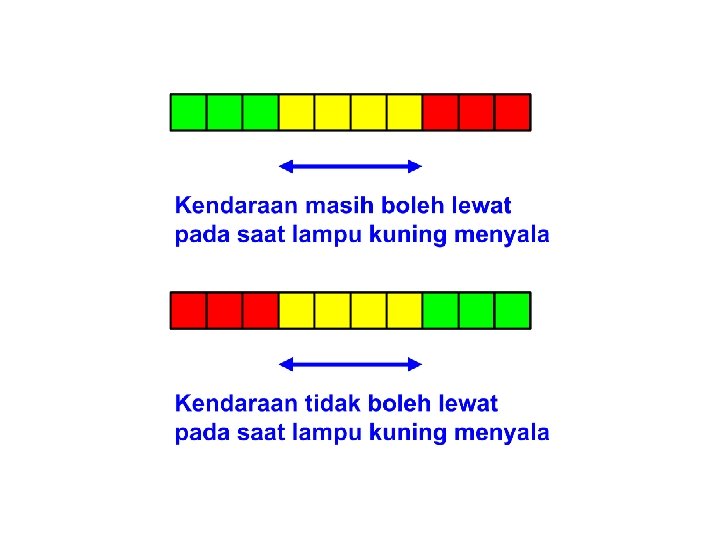
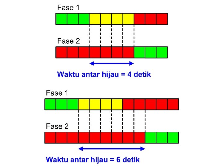
Cara-cara untuk meningkatkan kapasitas Simpang Bersinyal • Meminimalkan waktu antar-hijau Waktu antar-hijau diperlukan untuk menjamin keamanan kendaraan yang melewati simpang pada saat detik akhir hijau, agar tidak tertabrak kendaraan yang mendapatkan fase hijau berikutnya. Meminimalkan waktu hijau mendekatkan garis henti dengan pusat persimpangan.

Cara-cara untuk meningkatkan kapasitas Simpang Bersinyal • Larangan belok kanan Meningkatkan kapasitas akibat pengurangan fase. Namun harus dilakukan manajemen lalulintas untuk melayani kendaraan yang hendak belok kanan dengan menyediakan U-turn atau Rerouting.

Prinsip-prinsip desain simpang secara umum di Indonesia • Jari-jari tikungan berkisar antara 6 s/d 9 meter • Hindari jari-jari terlalu kecil kendala manuver bagi bus & truk • Fasilitas penyeberang jalan (zebra cross) 2, 5 s/d 5 meter sejarak 2 meter didepan garis henti • Panjang pelebaran harus lebih besar dari probabilitas panjang antrian terbesar

Prinsip-prinsip desain simpang secara umum di Indonesia • Jalur khusus berakhir pada awal panjang antrian terbesar • Jika arus lalulintas belok kanan cukup besar, perlu dibuatkan jalur khusus belok kanan dilengkapi dengan rambu dan marka yang sesuai