TROPICAL CYCLONE INNERCORE DYNAMICS PART 1 A LATENT

TROPICAL CYCLONE INNER-CORE DYNAMICS : PART 1. A LATENT HEAT RETRIEVAL AND ITS EFFECTS ON INTENSITY AND STRUCTURE CHANGE PART 2. THE IMPACTS OF EFFECTIVE DIFFUSION ON THE AXISYMMETRIZATION PROCESS Steve Guimond

Part 1: A Latent Heat Retrieval and its Effects on Intensity and Structure Change

Motivation • Main driver of hurricane genesis and intensity change is latent heat release • Observationally derived 4 -D distributions of latent heating in hurricanes are sparse • Most estimates are satellite based (i. e. TRMM) • Coarse space/time • No vertical velocity • Few Doppler radar based estimates • Water budget (Gamache 1993) • Considerable uncertainty in numerical model microphysical schemes • e. g. Mc. Farquhar et al. (2006) and Rogers et al. (2007)

Approach Refined latent heating algorithm (Roux 1985; Roux and Ju 1990) 1) 2) 3) 4) 5) 6) Observing System Simulation Experiment (OSSE) Examine assumptions/Uncover sensitivities Parameterization Present radar-derived retrievals Uncertainty estimates Impact study

Algorithm Examination Non-hydrostatic, full-physics, quasi cloud resolving (2 -km) MM 5 simulation of Hurricane Bonnie (1998; Braun 2006)

Structure of Latent Heat Ø Goal saturation using production of precipitation (Roux and Ju 1990) Ø Divergence, diffusion and offset are small and can be neglected

Structure of Latent Heat

Structure of Latent Heat

Magnitude of Latent Heat Ø Requirements Ø Temperature and pressure (composite eyewall, high-altitude dropsonde) Ø Vertical velocity (radar)

Putting it Together Positives… 1) Full radar swath coverage in various types of clouds (3 -D and 4 -D) 2) Only care about condition of saturation, not magnitude Uncertainties to consider… 1) 2) 3) 4) Estimating tendency term (Steady-state ? ) Quality of vertical velocity Thermo based on composite eyewall dropsonde Drop size distribution and feedback to derived parameters

Do we really need saturation? Aircraft (z = 1. 5 – 5. 5 km) Courtesy of Matt Eastin

Examining Uncertainties

Storage Parameterization

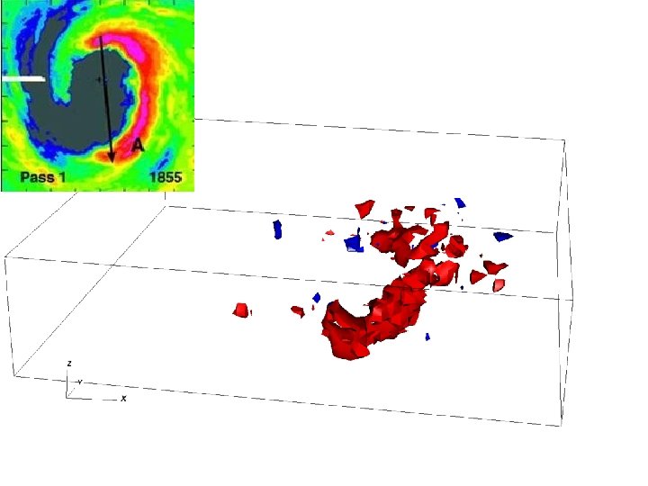
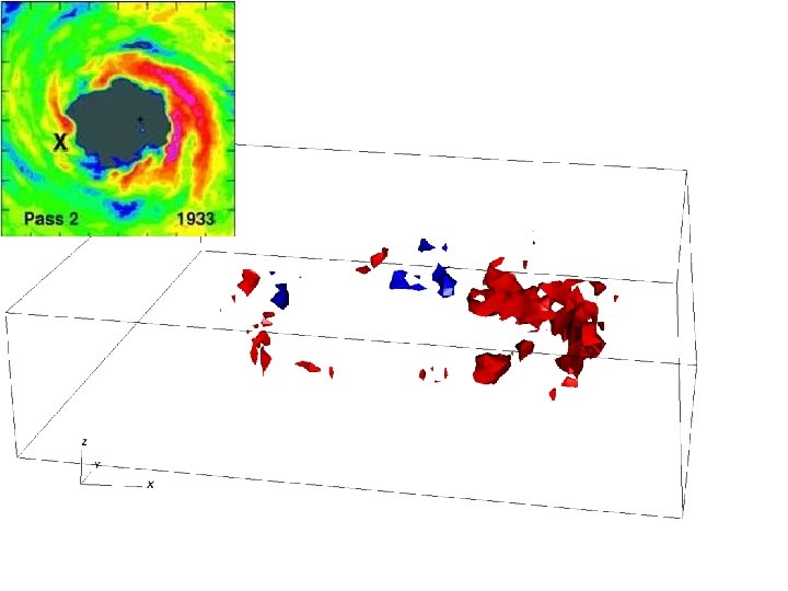
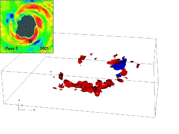
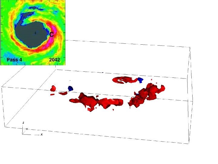
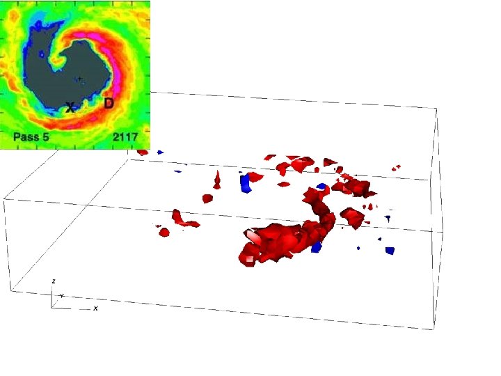
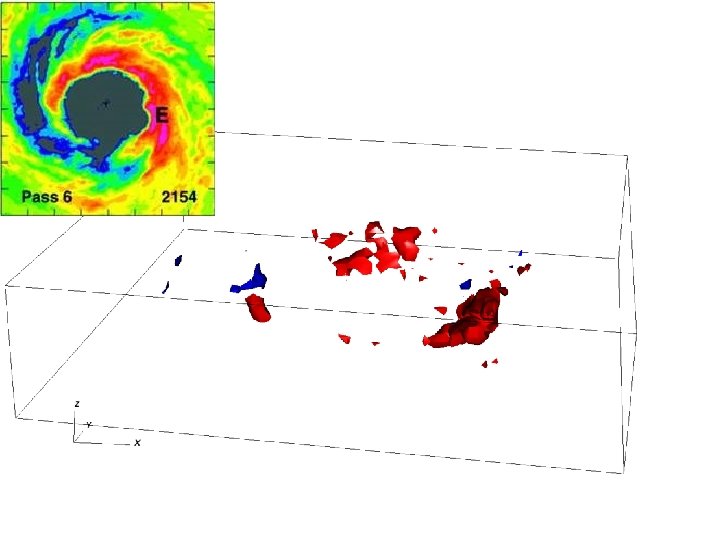
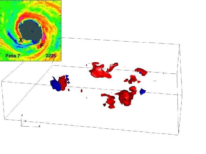
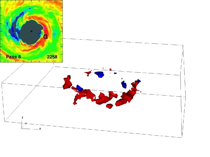
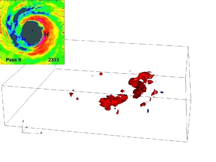
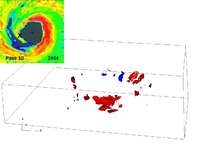
Observations • NOAA WP-3 D dual-Doppler radar observations of Hurricane Guillermo (1997; Reasor et al. 2009) • Variational analysis retrieves important variables (u, v, w) • 2 km x 1 km x ~34 min (10 snapshots = ~5. 5 h) • 2 -D particle data (Robert Black) in Katrina (2005) • Statistical fit between reflectivity and liquid water content

Hurricane Guillermo (1997) Figures from NHC report

Uncertainty Estimates Physical uncertainty Sampling uncertainty • Bootstrap (Monte Carlo method) • 95 % CI on mean = ~14%

Impact Study

Observations and Model • NOAA WP-3 D dual-Doppler radar observations of Hurricane Guillermo (1997; Reasor et al. 2009) • Variational analysis retrieves important variables (u, v, w) • 2 km x 1 km x ~34 min (10 snapshots = ~5. 5 h) • Nonlinear, compressible, Navier-Stokes solver; LANL’s HIGRAD model (Reisner et al. 2005) • Realistic setup • 2 km radar domain stretched to boundaries (1300 km 2), 71 levels • Full Coriolis • Reynolds OI high-resolution SST • ECMWF background • State-of-the-art cloud physics (Reisner and Jeffery 2009)

Vortex Initialization Airborne radar Environment (ECMWF)

Vortex Initialization Nudge momentum equations with first radar composite Thermal wind balance NHC ~ 958 h. Pa

Perturbations: Retrieval Run Force energy equation with retrievals (no heat from model) 5. 1 h t = 44 t = 10 t = 78 t=0 ∆t = 34

Perturbations: Freemode Run Initial water vapor forcing from heat retrieval conversion MICROPHYSICS 5. 1 h t = 44 t = 10 t = 78 t=0 ∆t = 34

Results: Integrated Error

Results: RMS Error

Results: Explained Variance

Comparisons: t = 0 h

Comparisons: t = 4. 67 h

Space & Time Averaged Structure Black = Obs; Green = Retrieval; Red = Freemode Tangential Wind Vorticity

Water Vapor Transport Retrieval Freemode

Conclusions: Part I • Improved latent heat of condensation algorithm • Computation of saturation (production of precipitation) performed well in numerical model setting • Need observational validation of computed saturation • Precipitation storage term shown to be important for retrievals • Developed parameterization based on advection • Uncertainty estimates for heating magnitudes • Insensitive to thermo, sensitive to vertical velocity • Physical and sampling uncertainty = ~ 15 – 25 % • Likely first 4 D view of latent heating in RI TC

Conclusions: Part I • Assuming saturation of entire TC inner-core inappropriate • Need to determine saturation state for |w| ≤ ~ 5 m/s • • For |w| > ~ 5 m/s saturation better assumption Latent heat retrieval simulation vs. freemode simulation • Retrievals: Reduce RMSE and explain 20 – 25 % more variance in wind • Larger errors in freemode run: 1) Transport of water vapor (advection & diffusion) 2) Microphysics scheme (limits on heat release)

Part 2: The Impacts of Effective Diffusion on the Axisymmetrization Process

Background/Motivation • Deeper understanding of dynamics responsible for TC intensification triggered by convection • Fundamental property = latent heat release • Nolan and Montgomery (2002; NM 02), Nolan and Grasso (2003; NG 03) and Nolan et al. (2007) • Azimuthal mean heating dominates • Pure asymmetric heating negligible impact • Vorticity anomalies extract energy before axisymmetrizing

Question to Consider • Nolan studies use simple, linear heating prescriptions • Does observational heating structure matter?

First Step • Reproduce nonlinear results of Nolan and Grasso (2003) • Able to reproduce the symmetric heating perturbation results to a LARGE degree. • Asymmetric heating case NOT SO EASY!

Numerical Model • HIGRAD (Reisner et al. 2005; Reisner and Jeffery 2009) • Equation set… • Discretization • Temporal semi-implicit (higher order an option) • Space finite volume on A-grid (non-staggered)

Numerical Model Setup • Attempt to mirror settings in WRF simulations of NG 03 • Dry • Same domain (600 km sq. box) and grid spacing (2 km) • Higher vertical resolution (71 levels) and model top (22 km) • Same Coriolis frequency (5. 0 x 10 -5 s-1) • Free slip of momentum and scalars on lower boundary • Relaxation to Jordan sounding on sides and top • Diffusion coefficients set to constant 40 m 2/s • Time step = 20 s, 6 h runs

Vortex on Cartesian Mesh (1) Stable vorticity profile from NM 02 (2) Compute u and v by solving Poisson equations (3) Baroclinic structure following NM 02 CLEAN VORTEX TO START

Vortex Initialization • How get balanced vortex at t = 0 ? • Solving for fields and starting model oscillations • Used nudging approach thermal wind balance 1 K WN 3

Symmetric vs. Asymmetric asymmetric -8. 8 x 10 -2 h. Pa -2. 7 x 10 -2 h. Pa NG 03: GR 10:

Understanding Discrepancy • Absolute Angular Momentum Budgets Secondary Circulation

Cause of Secondary Circulation

Cause of Secondary Circulation

Conclusions: Part 2 • Discrepancy with asymmetric NG 03 likely due to symmetric secondary circulation in basic-state vortex • NG 03 did not consider a secondary circulation • Secondary circulations are ubiquitous features of real TCs • Suggests impact of asymmetric mode important for more realistic numerically simulated TCs • Diffusion (sub-grid model) in HIGRAD responsible for 1)Significant, secondary circulation in vortex 2)Variability in vorticity anomalies produced from heating • Inherent uncertainty with diffusion parameterization in models at cloud resolving resolutions (e. g. 1 - 2 km) • Need turbulence resolving resolution (~ 50 m) simulations to understand role of asymmetric mode

Acknowledgments • Thanks to Ph. D Committee (Paul Reasor, Mark Bourassa, Bob Hart, Michael Navon, Chris Jeffery, Gerry Heymsfield, Ming Cai and X. Zou) • Jon Reisner for mentoring and modeling expertise • Dave Nolan for discussion, re-running WRF and figures. • Scott Braun, Robert Black, Dave Moulton and Matt Eastin for providing data, figures and assistance. • Funded by The Los Alamos National Laboratory through an LDRD project with Dr. Chris Jeffery the PI • Funding also from NASA ocean vector winds and NOAA grants

Future Work • Extend latent heating simulations out ~ 12 h and use Guillermo Day 2 observations for validation. • How does radial inflow affect asymmetric heat perturbation? • Accelerated, more vigorous axisymmetrization? • Excite instability in inner-core? • Turbulence modeling to reduce uncertainty in diffusion parameterization, impact of asymmetric heating.

Some Thoughts Radial flow and associated secondary circulation driven by dissipation Free slip along boundaries has been set correctly Wind components are barotropic in lowest layer. Thus, only a function of diffusive fluxes Why does diffusion/turbulence scheme play a different role in HIGRAD than WRF? Eddy diffusivity was set to same values as NG 03 WRF runs Stress tensor similar to WRF (also tried Laplacian in HIGRAD) Must come down to…design of numerical solution procedure HIGRAD WRF (1)Fully implicit in time (1)Time-split (2)A grid (2)C grid (3)No artificial filters (3)Divergence damping, etc.

Comparisons: t = 4. 25 h

Comparisons : t = 5. 42 h

Uncertainty Estimates • Bootstrap (Monte Carlo method) • Auto-lag correlation ~30 degrees of freedom • 95 % CI on mean = 101 - 133 K/h or ~14% • Physical uncertainty 8 K/h or ~27 % of mean (30 K/h)

AAM Budget for 1 K WN 3: t = 10 min θ’

AAM Budget for 1 K WN 3: t = 20 min

AAM Budget for 1 K WN 3: t = 30 min

AAM Budget 1 K WN 3: t = 40 min

AAM Budget for 1 K WN 3: t = 50 min

AAM Budget for 1 K WN 3: t = 60 min

Radial Flow: t = 30 min HIGRAD WRF

Radial Flow: t = 6 h HIGRAD WRF

With HIGRAD, I can reproduce these WRF results: (1)Min pressure perturbation for: Localized heat sources; Symmetric heat sources (2)Perturbation radial velocity for symmetric heat source (3)Vertical velocity for symmetric heat source (4)Perturbation tangential velocity for symmetric heat source (5)Perturbation vbar at surface for symmetric heat source