Tree Findera first step towards XML data mining

Tree. Finder：a first step towards XML data mining Advisor ： Dr. Hsu Graduate：Keng-Wei Chang Author ：Alexandre Termier Marie-Christine Michele Sebag

outline l Motivation Objective Introduction Example Formal background l Overview of the Tree. Finder system l Experimental results Conclusions Personal Opinion l l l

Motivation l l The construction of tree-based mediated schema for integrating multiple and heterogeneous sources of XML data. They consider the problem of searching frequent trees from a collection of treestructured data modeling XML data.

Objective l The Tree. Finder algorithm aims at finding trees, such that their exact or perturbed copies are frequent in a collection of labelled trees.

1. Introduction l They present a method that automatically extracts from a collection of labelled trees a set of frequent tree occurring as common(exact or approximate) trees embedded in a sufficient number of trees of the collection.

1. Introduction l Two step (i) a clustering of the input trees, l (ii) a characterization of each cluster by a set of 　　　　 　　 　　　 　 frequent trees. l l The important point that they are not looking for an exact embedding but for trees that may be approximately embedded in several input trees.

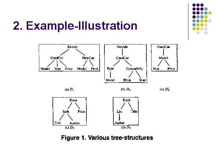
2. Example-Illustration

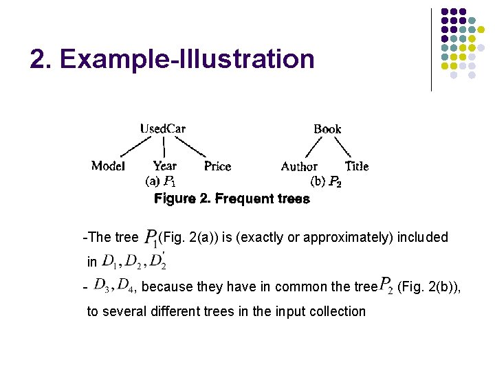
2. Example-Illustration -The tree (Fig. 2(a)) is (exactly or approximately) included in - , because they have in common the tree to several different trees in the input collection (Fig. 2(b)),

3. Formal background l Definition 1 (Labelled trees) A labelled tree is a pair (t, label) where l l (i) t is a finite tree whose nodes are in N (ii) label is a labeling function that assigns a label to each in t.

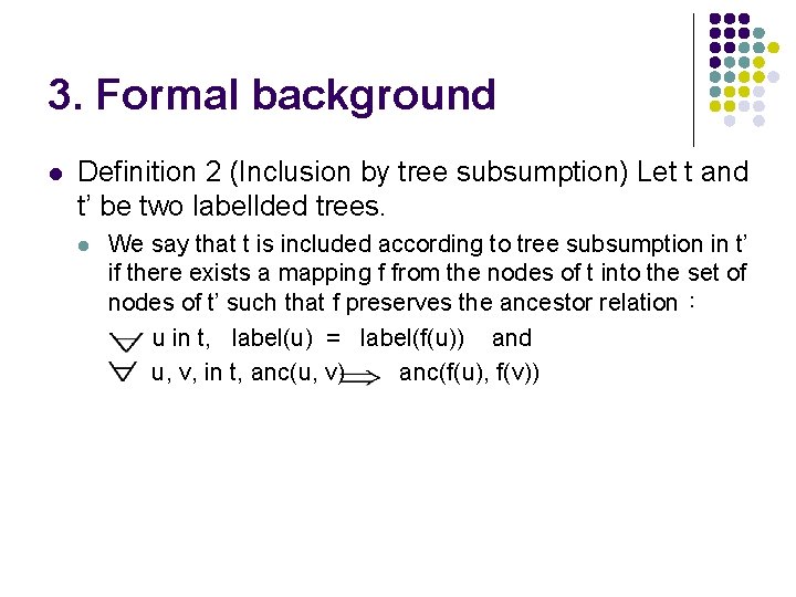
3. Formal background l Definition 2 (Inclusion by tree subsumption) Let t and t’ be two labellded trees. l We say that t is included according to tree subsumption in t’ if there exists a mapping f from the nodes of t into the set of nodes of t’ such that f preserves the ancestor relation： u in t, label(u) = label(f(u)) and u, v, in t, anc(u, v) anc(f(u), f(v))

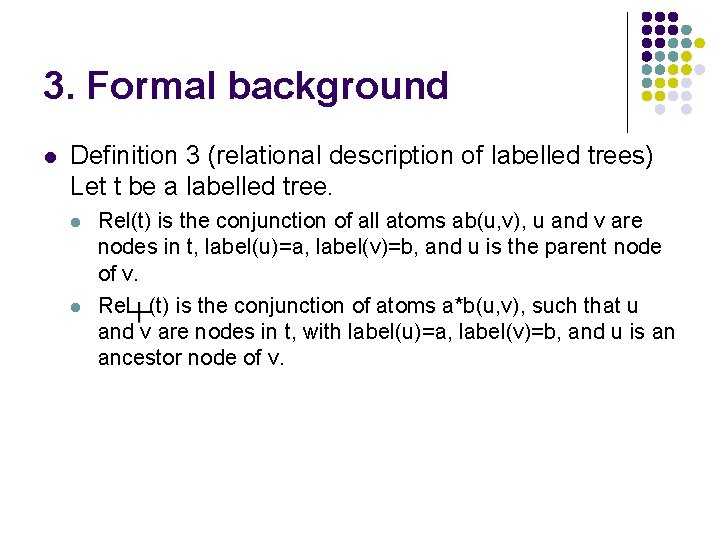
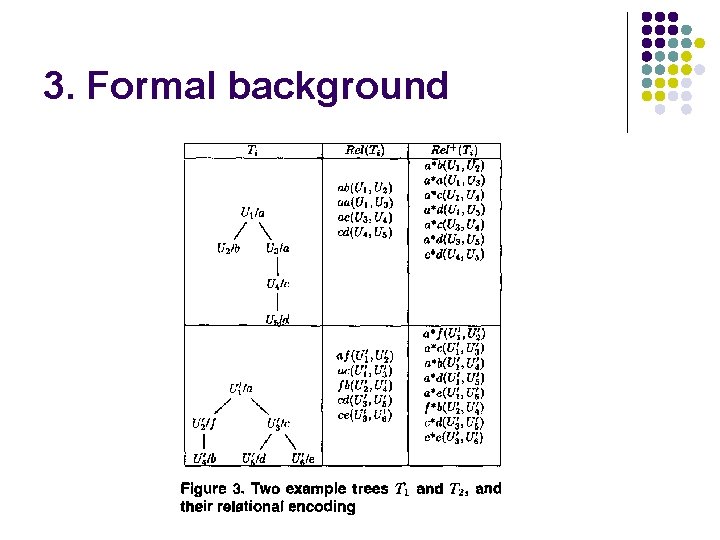
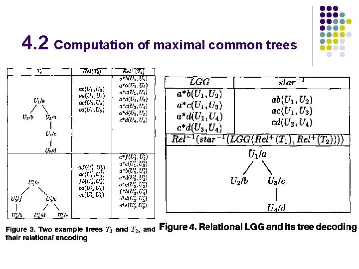
3. Formal background l Definition 3 (relational description of labelled trees) Let t be a labelled tree. l l Rel(t) is the conjunction of all atoms ab(u, v), u and v are nodes in t, label(u)=a, label(v)=b, and u is the parent node of v. Rel (t) is the conjunction of atoms a*b(u, v), such that u and v are nodes in t, with label(u)=a, label(v)=b, and u is an ancestor node of v.

3. Formal background

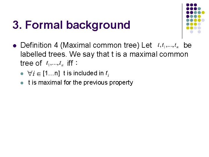
3. Formal background l Definition 4 (Maximal common tree) Let be labelled trees. We say that t is a maximal common tree of iff： l l 　　 [1…n] t is included in t is maximal for the previous property

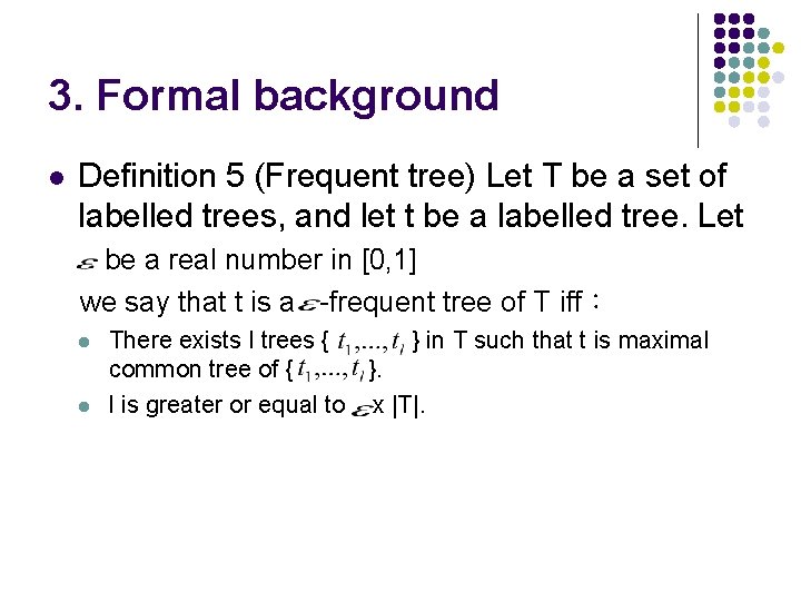
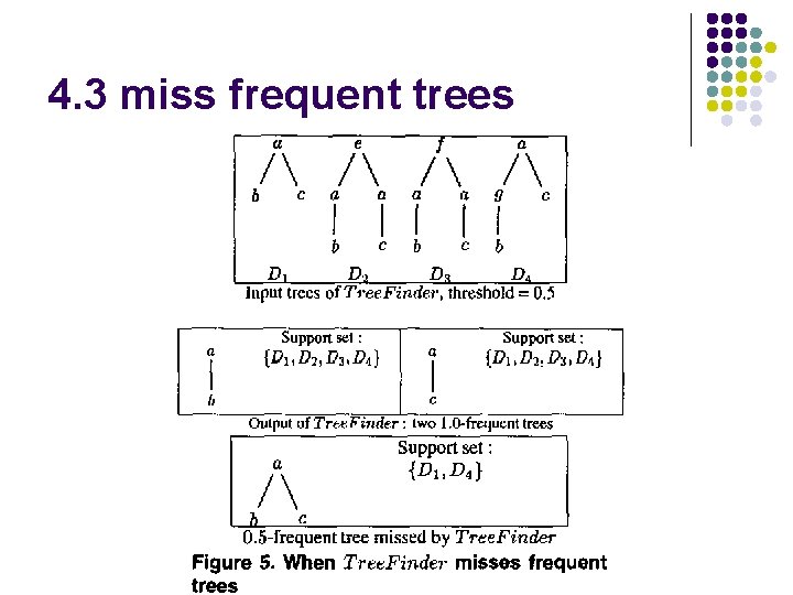
3. Formal background l Definition 5 (Frequent tree) Let T be a set of labelled trees, and let t be a labelled tree. Let be a real number in [0, 1] we say that t is a -frequent tree of T iff： l l There exists l trees { } in T such that t is maximal common tree of { }. l is greater or equal to x |T|.

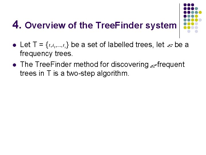
4. Overview of the Tree. Finder system l l Let T = { } be a set of labelled trees, let be a frequency trees. The Tree. Finder method for discovering -frequent trees in T is a two-step algorithm.

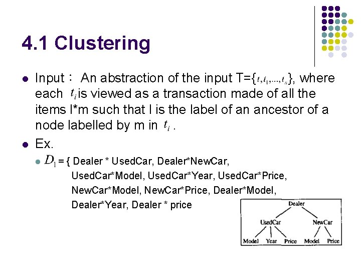
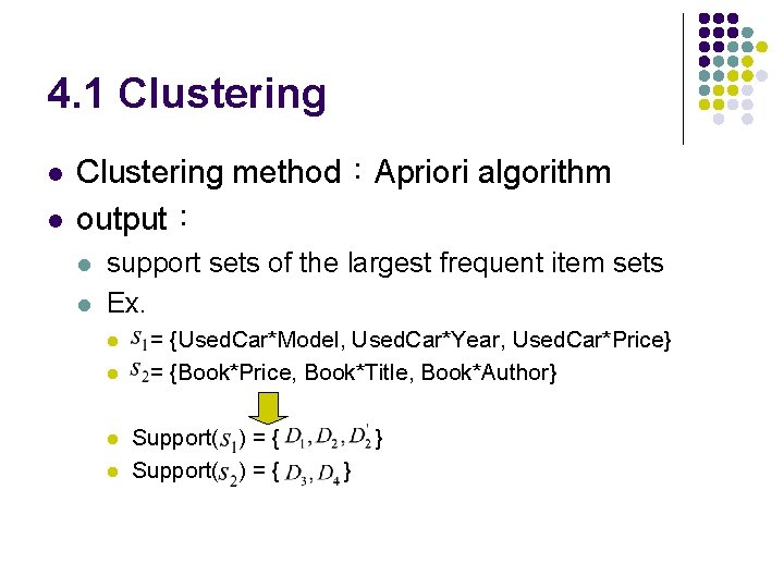
4. 1 Clustering l l Input： An abstraction of the input T={ }, where each is viewed as a transaction made of all the items l*m such that l is the label of an ancestor of a node labelled by m in. Ex. l = { Dealer * Used. Car, Dealer*New. Car, Used. Car*Model, Used. Car*Year, Used. Car*Price, New. Car*Model, New. Car*Price, Dealer*Model, Dealer*Year, Dealer * price

4. 1 Clustering l l Clustering method：Apriori algorithm output： l l support sets of the largest frequent item sets Ex. l l = {Used. Car*Model, Used. Car*Year, Used. Car*Price} = {Book*Price, Book*Title, Book*Author} Support( ) = { } }

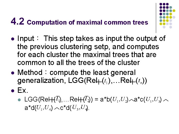
4. 2 Computation of maximal common trees l l l Input： This step takes as input the output of the previous clustering setp, and computes for each cluster the maximal trees that are common to all the trees of the cluster Method：compute the least generalization, LGG(Rel ( ), …Rel ( )) Ex. l LGG(Rel ( ), …Rel ( )) = a*b( a*d( ) c*d( ). ) a*c( )

4. 2 Computation of maximal common trees

4. 3 miss frequent trees

5. Experimental results l Tow goals l l Investigate Computational cost of Tree. Finder. Estimate the percentage of frequent trees missed by Tree. Finder.

5. 1 Experimental setting

5. 2 Empirical study of computational cost

5. 2 Empirical study of computational cost

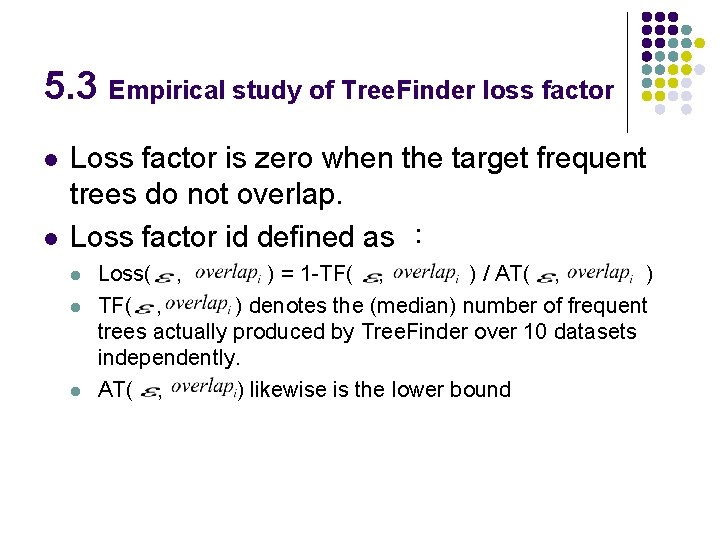
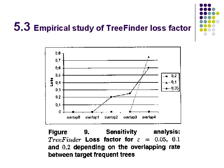
5. 3 Empirical study of Tree. Finder loss factor l l Loss factor is zero when the target frequent trees do not overlap. Loss factor id defined as ： l l l Loss( , ) = 1 -TF( , ) / AT( , ) TF( , ) denotes the (median) number of frequent trees actually produced by Tree. Finder over 10 datasets independently. AT( , ) likewise is the lower bound

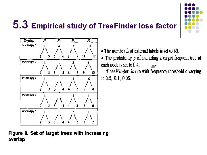
5. 3 Empirical study of Tree. Finder loss factor

5. 3 Empirical study of Tree. Finder loss factor

6. Conclusions l l The Tree. Finder achieves a more flexible and robust tree-mining and can detect trees that could not be discovered using a strict subtree inclusion. The main limitation of Tree. Finder is to be an approximate miner.

Personal Opinion l l Improve the LGG computational cost Overlap broblem