Traveling Salesperson Problem Steven Janke Colorado College Traveling

Traveling Salesperson Problem Steven Janke Colorado College
 A B C D A - 3 4 6 B")
Traveling Salesperson Problem (TSP) A B C D A - 3 4 6 B 2 - 5 2 C 7 4 - 3 D 5 6 7 - Optimization Problem: Find the least cost tour starting at A, traveling through the other three cities exactly once and returning to A. Decision Problem: Is there a TSP tour with cost less than k?

Sir William Hamilton 1805 - 1865 • Discovered quaternions in 1843 • Invented Icosian Game in 1857 • Hamiltonian Circuits T. P. Kirkman 1806 - 1895 In 1856, he published sufficient conditions for a polyhedral graph to have a Hamiltonian circuit.

Icosian Game 1857

Proctor & Gamble Contest 1962
")
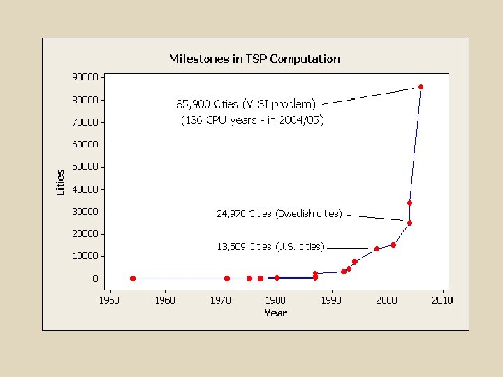
Twentieth Century History § 1931 -32 Merrill Flood, A. W. Tucker, Hassler Whitney (Princeton) pose the Traveling Salesperson Problem. § 1947 George B. Dantzig designs simplex method for linear programming. § 1954 Connection with the Assignment Problem established. § 1962 Dynamic programming formalized. § 1972 Karp proved TSP is NP-complete. § 1985 – 2008 Techniques leading to solving a 85, 000 -city problem

TSP Applications: q School Bus routing. q Robotic welding in the car industry. q Printed circuit board drilling and laser cutting of integrated circuits. q Genome sequencing. Finding most likely ordering of markers. q Job processing: Chemical plants – cost of setup to produce chemicals.

Mathais Herb ‘n Farm Cutler Hall Slocum El Pomar Packard Admissions Office Campus Tour Colorado College

Versions of the TSP: § Complete or Incomplete graph. § Symmetric vs. Asymmetric cost matrix. § Euclidean (Triangle inequality holds. ) § Upper Triangular cost matrix. § Circulant cost matrix. § Bipartite graph.

A A B C D A - 3 4 6 B 2 - 5 2 C 7 4 - 3 D 5 6 7 - D Traveling Salesperson Problem: Find the least cost tour starting at A, traveling through the other three cities exactly once and returning to A.

Generating Permutations: Recursion: A < BCD BDC CBD CDB DBC DCB B < ACD ADC CAD CDA DAC DCA C < ABD ADB BAD BDA DAB DBA D < ABC ACB BAC BCA CAB CBA Single exchange: ABCD BACD BCAD BCDA CBAD CABD ACDB CADB CDAB CDBA DCAB DACB ADBC DABC DBAC DBCA BDAC BADC ABDC

Naïve Algorithm 1. List all tours and their costs: A BCD A A BDC A A CBD A A CDB A A DBC A A DCB A = = = 18 19 15 15 24 19 2. Find a tour with minimum cost: A CBD A = 15 (one optimal tour)

Timing results for Naïve Algorithm: Cities Seconds Tours Sec/Tour 11 0. 50 3, 628, 800 1. 38 x 10 -7 12 5. 61 39, 916, 800 1. 41 x 10 -7 13 69. 12 479, 001, 600 1. 44 x 10 -7 Estimate for 17 cities: 34. 9 days (2. 09 x 1013 tours)
, then")
Complexity: § If there are n-1 cities (other than the home city A), then there are (n-1)! possible tours. § The naïve algorithm takes at least (n-1)! steps. § A random algorithm could possibly find an optimal tour in (n-1) steps. § Is there a deterministic algorithm that can find an optimal tour in a polynomial number of steps?
 TSP is NP-Complete. (That is, every other hard problem is reducible")
Theorem: (Karp, 1972) TSP is NP-Complete. (That is, every other hard problem is reducible to TSP. ) Open problem: Is there a polynomial time algorithm for TSP? If not, can you prove it? (In technical terms, does P = NP? ) Solving the open problem earns you $1, 000 from the Clay Mathematics Institute.

Approaches to the TSP: §Constant TSP: Analyze the cost matrix. § Linear Programming § Euclidean TSP: Probabilistic analysis. § Approximation algorithms § Search techniques ü Branch and Bound ü Dynamic Programming ü Genetic Algorithm ü Ant Colony

A Constant TSP B C D A BCD A = 22 A BDC A = 22 A B C D A - 1 3 5 B 10 - 6 8 C 8 2 - 6 D 9 3 5 - A CBD A = 22 A CDB A = 22 A DBC A = 22 A DCB A = 22
 The only cost matrices that give the same cost for all")
Theorem: (Constant TSP) The only cost matrices that give the same cost for all TSP tours are those with entries that satisfy: cij = ai + bj Sketch of Proof: § The set C of matrices with constant cost form a linear subspace. § The dimension of C is 2 n-1. § The matrices with either a single row of ones or a single column of ones belong to C and any set of 2 n-1 of them are linearly independent.

Constant TSP: a b c 1 6 - 1 3 5 4 0 10 - 6 8 2 2 8 2 - 6 3 4 9 3 5 -

Linear Program x 2 x 1+ x 2 = 5. 8 Feasible region Minimize: x 1+ x 2 Subject to: 2 x 1 + x 2 >= 5 x 1 + 2 x 2 >= 6 x 1 >= 0 x 2 >= 0 x 1+ x 2 = 1 x 1+ x 2 = 3. 67 x 1
 be a vector with an")
The TSP Polytope: § Let x = (xij ) be a vector with an entry 1 indicating that edge ij is included. Entry 0 indicates the edge is excluded. Hence the vector has length equal to the number of edges. § Let xt be the vector corresponding to the tour t. Polytope P = convex hull of {xt | t is a tour} Interestingly, dim P = |E| - |V| = n(n-3)/2 (Where E is the set of edges and V is the set of vertices. )

Linear Programming formulation of the TSP: Relaxation of the Linear Program: Additional contraints:

Euclidean TSP: The triangle inequality holds for the distance matrix. For any three cities A, B, C, AB + BC >= AC (Note that the distance measure could be something other than the Euclidean distance. ) For the Euclidean TSP, the tour does not cross itself. The Euclidean TSP is still NP-Complete, but there approximation algorithms.

Edge Crossings in Geometric TSP A B e C D Ae + e. B >= AB and Ce + e. D >= CD AD + CB >= AB + CD

Euclidean TSP on the unit cube

Minimum Spanning Tree: Pick next smallest edge connected to partial tree but not forming a cycle. 11 D 6 9 E 7 2 4 10 A C 5 7 9 B

Minimum Spanning Tree Algorithm: 11 D 6 9 E 7 2 4 10 A C 5 7 9 B To form a TSP tour, trace the minimum spanning tree twice using short cuts if possible. This gives A-E-B-C-D-A. The cost of this tour is 31. The spanning tree has cost 19.

Euclidean Approximation Guarantee: § Let OPT = cost of optimal TSP tour. MST = cost of minimum spanning tree. RMT = cost of route derived from minimum spanning tree. § The optimal TSP tour minus the last edge is a minimum spanning tree, so MST < OPT. § Then RMT <= 2*MST <= 2*OPT § With a little more care the shortcuts can be optimized to give: RMT <= 1. 5*OPT § Recently an algorithm scheme was discovered that gives RMT <= (1+e)*OPT for arbitrary e > 0

Approximations for the General TSP: Can an approximation algorithm find a tour that is, say, within 110% of the optimal route? For an approximation algorithm A and TSP instance I, let A(I) be the cost of the tour it generates and let OPT(I) be the optimal cost. Bottom line: No polynomial time algorithm A can guarantee that for all instances I of TSP, A(I) < r OPT(I) for any constant r, unless P=NP. Nevertheless, there are “rules” (called heuristics) that help find good, if not optimal, TSP tours: üNearest Neighbor üDissection üNearest Insertion üTour Improvement

A Search Tree B C C D B D D B C Little work required. D C D B C Total nodes: 1+ (n-1)(n-2) + … + (n-1)! (For 4 cities, there are 10 nodes. ) B

A B C C D D B C C Branch and Bound techniques possibly reduce the number of nodes visited.

Branch and Bound Technique Add A to the possible list and assign arbitrary cost. While the possible list is not empty do: - Select node with smallest estimated cost and remove from list. - Generate children of selected node and add to list. - If children complete a tour, update optimal tour, otherwise estimate cost of completed tour using this child. - If estimated cost is greater than current optimal, remove node from list. Estimate must be a lower bound on the cost and is called the bounding function. Technique depends on how accurate estimate is.
 : Each node i in the search tree represents")
A Possible Bounding Function B(i) : Each node i in the search tree represents a partial tour. Those cities not in the partial tour form a set of “remaining” cities. C 1 = cost of partial tour. C 2 = sum of the minimum edges into each remaining city. B(i) = C 1 + C 2 B(i) <= Cost of any tour containing the partial route.

Shortest Campus Tour: 1281 seconds Mathais Herb ‘n Farm Tutt Library Cutler El Pomar Elapsed time: 1. 05 seconds Total nodes visited: 710, 050 Slocum Armstrong
 Cities Time")
Timing Results for Branch and Bound Algorithm (Average of 3 Instances. ) Cities Time (Sec) Visited Nodes Total Nodes 15 0. 05 26, 599 8. 7 x 10¹⁰ 20 0. 33 188, 360 1. 2 x 10¹⁷ 25 11. 86 5, 294, 282 6. 2 x 10²³ 17 City Admission Tour: 1. 05 seconds (710, 050 nodes visited out of 2 x 10¹³)

Ant Colony Optimization § Ants find shortest path to food. § They deposit pheromone on trail. § Trails with most pheromone get most ants. § Basic searching behavior has random character.

Ant Colony Optimization Algorithm for TSP: Place some ants at each city and iterate the following: r s 1. While at city i, an ant calculates aij = cij / d ij where c ij is the amount of pheromone and d ij is the distance between i and j. 2. Each ant selects a city not already visited with probabilities proportional to the aij. 3. After all ants have built a tour, evaporate some fraction of the existing pheromone. 4. Each ant deposits an amount of pheromone inversely proportional to the length of their tour.

Mathais Ant Campus Tour: 1291 seconds Herb ‘n Farm Tutt Library Cutler El Pomar Elapsed time: 1. 6 seconds Ant Tours: 34, 000 Slocum Armstrong
")
Line drawings with TSP routes: (Robert Bosch and Craig Kaplan)
 - Lawler, Lenstra, Rinnoooy Kan, Shmoys §")
References: § The Traveling Salesman Problem (1985) - Lawler, Lenstra, Rinnoooy Kan, Shmoys § The Traveling Salesman Problem and its Variations (2002) - Gutin, Punnen § The Traveling Salesman Problem: A Computational Study (2006) - Applegate, Bixby, Chvatal, Cook

Dynamic Programming Algorithm: A – BCD A – BCD EFG – A EGF – A FGE – A FEG – A GFE – A GEF – A FEG Optimal A – CBD FEG – A g(i, S) = shortest path from i through vertices in S ending at A. g(i, S) = min { c i, j + g(j, S - {j}) } j in S Optimal tour = g(A, {all vertices}-A) Steps: n 2 x 2 n
- Slides: 42