Trapezoidal Maps Notes taken from CG lecture notes

Trapezoidal Maps Notes taken from CG lecture notes of Mount (pages 60 -69) Course page has a copy

Trapezoidal Maps • A randomized point location scheme, with (expected) query O(logn), space O(n), and construction time O(nlogn). • The bounds holds for any subdivision. • Simpler to implement, and its constant factors are better than Kirkpatrick’s. • The algorithm is based on trapezoidal maps, or decompositions, also encountered earlier in triangulation.

Trapezoidal Maps • S={s 1, s 2, . . . , sn} is the set of line segments – segments don’t intersect, but can touch – assuming that if the endpoints are not touching, the x-coordinates of their segments have distinct endpoints • Trapezoidal map results when a bullet is shot upwards and downwards from each vertex until it hits another segment of S. – to avoid infinite bullet paths, we assume that S is contained within a large bounding box.

• all faces are trapezoids with vertical sides • the left or the right side might be degenerate

Size of the map of n line segments Claim: Given a polygonal subdivision with n segments, the resulting trapezoidal map has at most 6 n+4 vertices and 3 n+1 trapezoids. • bound on the vertices – each vertex shoots two bullets, thus creating two vertices; each segment has two endpoints; the bounding rectangle has 4 vertices – Total number of vertices: 2 n (endpoints)+2. 2 n (bullet points) + 4 = 6 n+4

Size of the maps of n line segments Claim: Given a polygonal subdivision with n segments, the resulting trapezoidal map has at most 6 n+4 vertices and 3 n+1 trapezoids. • bound on the trapezoids : – each segment realizes the following • left endpoint of s supports two trapezoids from the left. • right endpoint of s supports one trapezoid from the left • total is 3 – leftmost trapezoid is not bounded by any point from the left – number of trapezoids is at most 3 n+1

Data structure for each trapezoid

We also store the pointers to the neighboring trapezoids (no more than 4)

Each trapezoid is determined by 4 entities • a segment on the top • a segment on the bottom • a bounding vertex on the left • a bounding vertex on the right We also store the pointers to the neighboring trapezoids (no more than 4)

The data structure allows. . . tracing a polygonal chain C through the trapezoidal map of S in O(|C| + k) where k is the number of trapezoids intersected by C, provides C does not properly intersect any segment of S. (We are assuming that the starting trapezoid is given)

Incremental algorithm • Start with the bounding rectangle (starting trapezoid) • We then add the segments in random order one at a time. As each segment is added, update the trapezoidal map. • Si = set of first i random segments Ti = the resulting trapezoidal map • When a new segment si is added, we perform the following operations on Ti-1. – Find the trapezoids of Ti-1 that contain the left and the right endpoint of si. – Trace the line segment si from left to right, determining which trapezoids it intersects. – Go back to these trapezoids and fix them. – The left and the right endpoint of si need to have bullets fixed from them. – One of the earlier bullet path might hit this line segment. We need to trim this bullet path.

X X X

• Observe that the structure does not depend on the order in which the segments are added. • Ignoring the time spent on locating the endpoint si, the time it takes to insert si is O(ki) where ki is the number of created trapezoids.

Expected time to build Tn • Later we will argue that O(log n) time is needed on an average to locate the trapezoid containing the left endpoint of each new segment. • We will show that the expected value of ki, E(ki) is O(1). • This results in an O(nlogn) expected time algorithm for the incremental construction of the trapezoidal map of n segments.

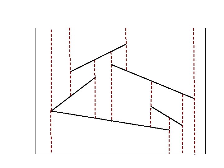
Inserting si • Worst case situation: Tracing cost is O(n) Starting point

Inserting si • On an average each insertion results in a constant # of trapezoids being created • Intuition: – Short segment might not intersect very many trapezoids – long segment may cut many trapezoids, but it shields later segments from cutting through many trapezoids.

Lemma A: E(ki) is O(1). • The analysis will be based on a backward analysis. Here Ti denote the map after si is inserted. • Since each segment is inserted at random, each segment has an equal probability of 1/i to be the last segment to have been added. • Let δ(Δ, s)=1 if segment s defines one of the sides of Δ, otherwise δ(Δ, s)=0. • Therefore

Showing that E(ki) is O(1). • Instead of counting the number of trapezoids that depend on each segment, we count the number of segments each trapezoid depend on • Therefore • Since each trapezoid is defined by 4 segments, E(ki) ≤ 1/i*|Ti|*4 = 1/i*O(i)*4 = O(1)

Incremental algorithm • Start with the bounding rectangle (starting trapezoid) • We then add the segments in random order one at a time. As each segment is added, update the trapezoidal map. • Si = set of first i random segments Ti = the resulting trapezoidal map • When a new segment si is added, we perform the following operations on Ti-1. – Find the trapezoids of Ti-1 that contain the left and the right endpoint of si. – Trace the line segment si from left to right, determining which trapezoids it intersects. – Go back to these trapezoids and fix them. – The left and the right endpoint of si need to have bullets fixed from them. – One of the earlier bullet path might hit this line segment. We need to trim this bullet path.

Running time of inserting si has two parts • Query time : one point location in Ti-1 • Tracing time through the trapezoids in Ti-1 – We have seen that this takes expected O(1) time.

Step: Find the trapezoid in Ti-1 that contains the left endpoint of si • Point Location Structure: The data structure is a rooted directed acyclic graph. Each node has either two or zero outgoing edges. Each leaf (node with zero outgoing edge) stores a trapezoid in the map. The other nodes are internal nodes that facilitate the point location search. As we will see later, this search structure is not a binary tree.

Two types of internal nodes • x-nodes – each x-node contains the x-coordinate x 0 of an endpoint of one of the segment. The search takes the left branch if the x-coordinate of the query point q is less than x 0, otherwise it takes the right branch. • y-nodes – each y-node contains a pointer to a line segment s of Si. The left and the right children correspond to whether the query point is below or above the line segment s. In this case the x-coordinate of the query point lies between the x-coordinates of the endpoints of s.

x 0 x-node s y-node

Few steps of the algorithm • s 1 is added T 1 2 s 1 1 p 1 q 1 11 4 D 1 s 1 41 3 31 21

Few steps of the algorithm Perform search on D 1 to locate the trapezoid that contains the left point p 2. • s 2 is added T 1 2 s 1 1 p 1 3 p 1 q 1 p 2 4 D 1 q 1 11 s 1 q 2 31 41 21

Few steps of the algorithm • s 2 is added (intermediate stage) p 1 q 1 11 2 s 1 1 p 1 3 q 1 p 2 3’ s 1 q 12 4’ 4 p 12 q 2 31 21 1 3’ 1 4’ 41

Few steps of the algorithm • s 2 is added (Final) p 1 q 1 11 2 s 1 1 p 1 3 q 1 p 2 6 7 s 2 5 q 2 s 1 4 q 2 p 2 s 2 21 41 s 2 31 7 5 6

Analysis of point location structure • Three cases of how the end points of si can lie inside a trapezoid.

Analysis of point location structure • Local modifications after si is added. More comparisons are needed for point location inside the old trapezoid. Point location needs 2 comparisons (worst case} Point location needs 2 comparisons (worst case) Point location needs 3 comparisons (worst case)

Analysis of Tn • Expected size of Tn is O(n) – The number of new nodes is proportional to the number of newly created trapezoids. – The expected number of new trapezoids after an insertion is O(1) – Expected total size is O(n).

Claim: Expected query time in Tn is O(logn) – Consider one query point q, chosen arbitrarily. – Let us consider how q moves incrementally through the structure with the addition of new line segment. – Let Δi be the trapezoid q lies after the insertion of i segments. – If Δi-1 = Δi, insertion of si did not affect the trapezoid that q was in. – Suppose Δi-1≠ Δi. In this case q must be relocated. – In the worst case we need to make 3 comparisons to relocate (i. e. q falls as much as 3 levels) – The probability that q changes at the ith step is 4/i. – The expected length of a path is at most 3. 4. (1+1/2+1/3+. . . + 1/n) = 12 Hn = O(logn)

Some useful Lemmas • Lemma B: For any q, if we know that q ε Δj where Δj ε Tj, the expected cost of locating q in Tk, k ≥ j is at most 12. (Hk – Hj) which is O(log k/j). – This follows easily from the query time analysis

Some useful Lemmas • Lemma C: Let R be a random subset of S, |R|=r. Let Z be the intersections between T(R) and SR. The expected value of Z is O(n-r). Proof: For any s ε SR, the number of intersections between s and the trapezoidal map of R, T(R) is deg(s, T(RU{s}))

Seidel’s Trapezoidal Partitioning Algorithm Define log(i)n = log. . . logn (i times) log*n = max(h|log(h)n ≥ 1} N(h) = ceiling(n/log(h)n); N(0)=1 Generate a random order s 1, s 2, . . . , sn. Let Si={ s 1, s 2, . . . , si} • T(Si): Trapezoidal map of Si • D(Si): Point location data structure for T(Si) • •

Algorithm 1. Generate T(S 1) and D(S 1) 2. For h = 1 to log*n do (a) for i = N(h-1) + 1 to N(h) do Insert segment si, producing T(Si) and D(Si) from T(Si-1) and D(Si-1). (b) Trace the edges of polygon P through T(N(h)) to locate the endpoints of all sj, j > N(h). 3. i = N(log*n) + 1 to n do Insert si, producing T(Si) and D(Si) from T(Si-1) and D(Si -1).

Algorithm Analysis 1. Generate T(S 1) and D(S 1) Takes O(1) time 2. For h = 1 to log*n do (a) for i = N(h-1) + 1 to N(h) do Insert segment si, producing T(Si) and D(Si) from T(Si-1) and D(Si-1). ≤ N(h)*[ O(1) (Lemma A) + O(log(N(h)/N(h-1)) (Lemma B) ] i. e N(h)*[O(1) + O(log(n/N(h-1))) i. e N(h)*[O(1) +O( log(n/ceiling(n/log(h-1)n)))] i. e N(h)*O(loglog(h-1)n) i. e N(h)*O(log(h)n) = O(n). (b) Trace the edges of polygon P through T(N(h)) to locate the endpoints of all sj, j > N(h). O(n) by Lemma C

Algorithm 1. Generate T(S 1) and D(S 1) 2. For h = 1 to log*n do (a) for i = N(h-1) + 1 to N(h) do Insert segment si, producing T(Si) and D(Si) from T(Si-1) and D(Si-1). (b) Trace the edges of polygon P through T(N(h)) to locate the endpoints of all sj, j > N(h). 3. i = N(log*n) + 1 to n do Insert si, producing T(Si) and D(Si) from T(Si-1) and D(Si -1). = O(n)* O(log(n/N(log*n))) (Lemma A and B) i. e O(n)*O(1) = O(n)

Finally • Theorem: Let S be a set of n segments that form a simple polygon. Then – One can build T(S) and D(S) in O(nlog*n) time – Expected size of D(S) is O(n) – Expected query time for any q in D(S) is O(log n) • The same results holds if P is a connected polygonal subdivision. In step 2(b) of the algorithm, a graph traversal algorithm is used to trace P through T(N(h)).

Planar Subdivision

Degeneracy s 1 s 2

Degeneracy s 1 s 2

Degeneracy s 1 This trapezoid has empty interior. s 2

Degeneracy s 1 s 3 s 2

Degeneracy s 1 s 3 s 2 Total number of trapezoids (including the degenerate ones) is still at most 3 n+1