Transportation Problems Initial Solution Mr Harish G Nemade
 Mr. Harish G. Nemade Dept. of Mathematics Dhanaji Nana Mahavidyalaya,")
Transportation Problems (Initial Solution) Mr. Harish G. Nemade Dept. of Mathematics Dhanaji Nana Mahavidyalaya, Faizpur

Outline • Introduction • Solution Procedure for Transportation Problem • Finding an Initial Feasible Solution • Finding the Optimal Solution • Special Cases in Transportation Problems • Maximisation in Transportation Problems • Exercises

Operation Research The main typical issues in OR : v. Formulate the problem v. Build a mathematical model § Decision Variable § Objective Function § Constraints v. Optimize the model

Introduction Transportation models deal can be formulated as a standard LP problem. Typical situation shown in the manufacturer example q Manufacturer has three plants P 1, P 2, P 3 producing same products. q From these plants, the product is transported to three warehouses W 1, W 2 and W 3. q Each plant has a limited capacity, and each warehouse has specific demand. Each plant transport to each warehouse, but transportation cost vary for different combinations. The problem is to determine the quantity each warehouse in order to minimize total transportation costs.

Solution Procedure for Transportation Problem § § § Conceptually, the transportation is similar to simplex method. Begin with an initial feasible solution. This initial feasible solution may or may not be optimal. The only way you can find it out is to test it. If the solution is not optimal, it is revised and the test is repeated. Each iteration should bring you closer to the optimal solution.

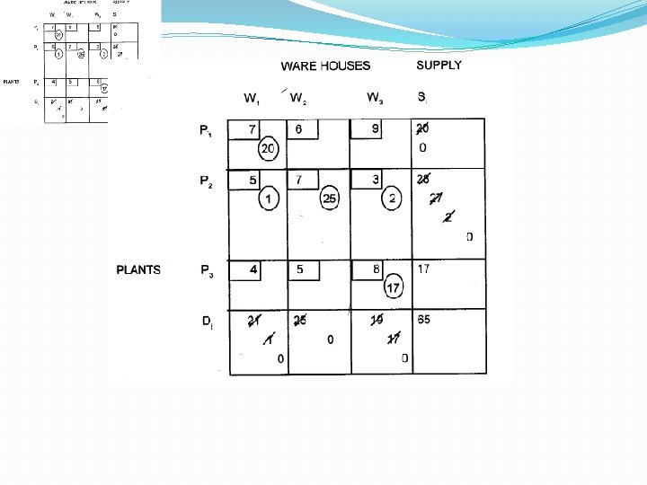
Solution Procedure for Transportation Problem The format followed in the above table will be used throughout the unit. • Each row corresponds to a specific plant and each column corresponds to a specific warehouse. • Plant supplies are shown to the right of the table and warehouse requirements are shown below the table. • The larger box (also known as cells) at the intersection of a specific row and column will contain both quantity to be transported and per unit transportation cost. • The quantity to be transported will be shown in the centre of the box and will be encircled and the per unit transportation cost is shown in the smaller rectangular box at the left hand side corner.

Finding an Initial Feasible Solution There a number of methods for generating an initial feasible solution for a transportation problem. Consider three of the following (i) North West Corner Method (ii) Least Cost Method (iii) Vogel’s Approximation Method
 The simplest of the procedures used to generate an")
North West Corner Method (NWCM) The simplest of the procedures used to generate an initial feasible solution is NWCM. It is so called because we begin with the North West or upper left corner cell of our transportation table. Various steps of this method can be summarised as under. Step 1 Select the North West (upper left-hand) corner cell of the transportation table and allocate as many units as possible equal to the minimum between available supply and demand requirement i. e. , min (S 1, D 1). Step 2 Adjust the supply and demand numbers in the respective rows And columns allocation.
 If the supply for the first row is exhausted, then move")
Step 3 (a) If the supply for the first row is exhausted, then move down to the first cell in t he second row and first column and go to step 2. (b) If the demand for the first column is satisfied, then move horizontally to the next cell in the second column and first row and go to step 2. Step 4 If for any cell, supply equals demand, then the next allocation can be made in cell either in the next row or column. Step 5 Continue the procedure until the total available quantity id fully allocated to the cells as required.

Remark 1: The quantities so allocated are circled to indicated, the value of the corresponding variable. Remark 2: Empty cells indicate the value of the corresponding variable as zero, I. e. , no unit is shipped to this cell. To illustrate the NWCM, As stated in this method, we start with the cell (P 1 W 1) and Allocate the min (S 1, D 1) = min (20, 21)=20. Therefore we allocate 20 Units this cell which completely exhausts the supply of Plant P 1 and leaves a balance of (21 -20) =1 unit of demand at warehouse W 1
 At this stage")
Now, we move vertically downward to cell (P 2 W 1) At this stage the largest allocation possible is the (S 2, D 1 – 20) =min (28, 1)= 1. This allocation of 1 unit to the cell (P 1 W 2). Since the demand of warehouse W 2 is 25 units while supply available at plant P 2 is 27 units, therefore, the min (27 -5) = 25 units are located to the cell (P 1 W 2). The demand of warehouse W 2 is now satisfied and a balance of (27 -225) = 2 units of supply remain at plant P 2. Moving again horizontally, we allocated two units to the cell (P 2 W 3) Which Completely exhaust the supply at plant P 2 and leaves a balance of 17 units to this cell (P 3, W 3). . At this, 17 Units ae availbale at plant P 3 and 17 units are required at warehouse W 3. So we allocate 17 units to this cell (P 3, W 3). Hence we have made all the allocation. It may be noted here that there are 5 (+3+1) allocation which are necessary to proceed further. The initial feasible solution is shown below. The Total transportation cost for this initial solution is Total Cost = 20 x 7 +1 X 5 + 25 x 7 + 2 X 3 + 17 + 8 = Rs. 462

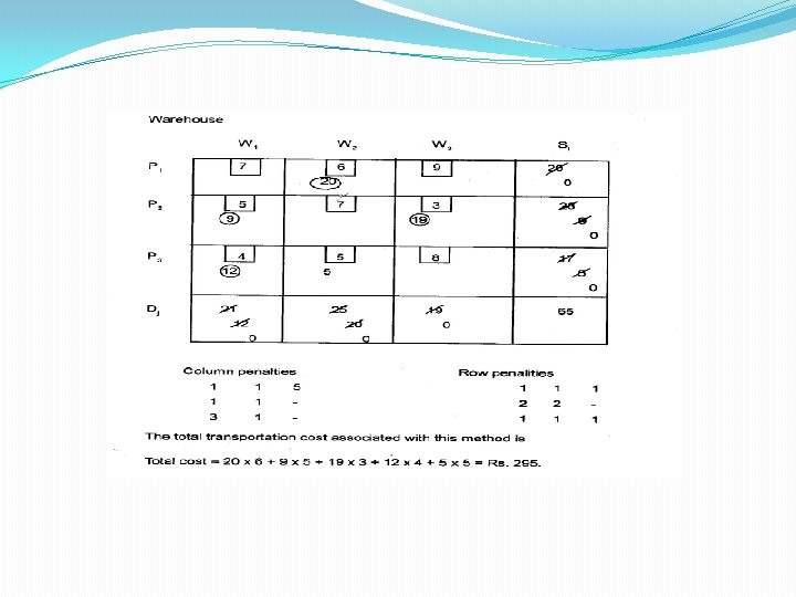
Least Cost Method The allocation according to this method is very useful as it takes into consideration the lowest cost and therefore, reduce the computation as well as the amount of time necessary to arrive at the optimal solution. Step 1 (a) Select the cell with the lowest transportation cost among all the rows or columns of the transportation table. (b) If the minimum cost is not unique, then select arbitrarily any cell with this minimum cost. Step 2 Allocate as many units as possible to the cell determined in Step 1 and eliminate that row (column) in which either supply is exhausted or demand is satisfied.

Repeat Steps 1 and 2 for the reduced table until the entire supply at different plants is exhausted to satisfied the demand at different warehouses.
 This method is preferred over the other two methods because")
Vogel’s Approximation Method (VAM) This method is preferred over the other two methods because the initial feasible solution obtained is either optimal or very close to the optimal solution. Step 1: Compute a penalty for each row and column in the transportation table. Step 2: Identify the row or column with the largest penalty. Step 3: Repeat steps 1 and 2 for the reduced table until entire supply at plants are exhausted to satisfy the demand as different warehouses.
- Slides: 16