Transportation Engineering I Lec03 Horizontal Alignment Sight Distances

Transportation Engineering I Lec-03 Horizontal Alignment & Sight Distances Dr. Attaullah Shah

Sight Distance For operating a motor vehicle safely and efficiently, it is of utmost importance that drivers have the capability of seeing clearly ahead. Therefore, sight distance of sufficient length must be provided so that the drivers can operate and control their vehicles safely. Sight distance is the length of the highway visible ahead to the driver of the vehicle

Aspects of Sight Distance • The distances required by motor vehicles to stop. • The distances needed for decisions at complex locations • The distances required for passing and overtaking vehicles, applicable on two lane highways • The criteria for measuring these distances for use in design.

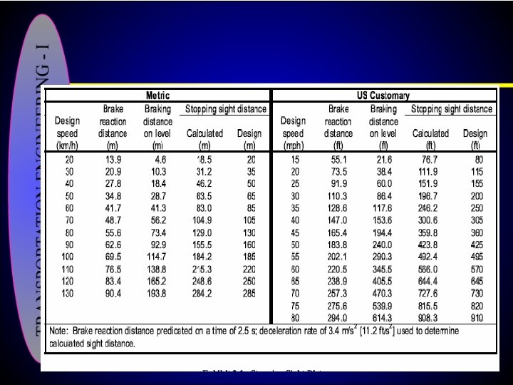
Stopping Sight Distance At every point on the roadway, the minimum sight distance provided should be sufficient to enable a vehicle traveling at the design speed to stop before reaching a stationary object in its path. Stopping sight distance is the aggregate of two distances: • brake reaction distance and • braking distance.

Brake reaction time It is the interval between the instant that the driver recognizes the existence of an object or hazard ahead and the instant that the brakes are actually applied. Extensive studies have been conducted to ascertain brake reaction time. Minimum reaction times can be as little as 1. 64 seconds: 0. 64 for alerted drivers plus 1 second for the unexpected signal. Some drivers may take over 3. 5 seconds to respond under similar circumstances. For approximately 90% of drivers, including older drivers, a reaction time of 2. 5 sec is considered adequate. This value is therefore used in Table 3. 1

The braking distance of a vehicle on a roadway may be determined by the formula Equation (1) d = braking distance (ft) or (m) v = initial speed (ft/s) or (m/s) a = deceleration rate, ft/s² (m/s²)

Studies (Fambro et a. I. , 1997) document that most drivers decelerate at a rate greater than 4. 5 m/s² (14. 8 ft/s²) when confronted with an urgent need to stop for example, when seeing an unexpected object in the roadway. Approximately 90 percent of all drivers displayed deceleration rates of at least 3. 4 m/s² (11. 2 ft/s²).

Such deceleration rates are with in a driver's capability while maintaining steering control and staying in a lane when braking on wet surfaces. Most vehicle braking systems and tire pavement friction levels are also capable of providing this level. Therefore, a deceleration rate of 3. 4 m/s² (11. 2 ft/s²) is recommended as a threshold for determining stopping sight distance (AASHTO, 2004).

Design Values The sum of the distance traversed during the brake reaction time and the distance to brake the vehicle to a stop is the stopping sight distance. The computed distances for wet pavements and for various speeds at the assumed conditions are shown in Exhibit 3 1 and were developed from the following equation:

Equation 2 where tr is the driver reaction time (sec). If speed is given in miles per hour or kilometer per hour, Equation (2) can be rewritten as

Note that the units for S are in feet and V is in miles per hour, assuming that 1 ft/sec = 0. 682 mph (or 1. 466 ft/sec = 1 mph).

In computing and measuring stopping sight distances, the height of the driver's eye is estimated to be 1, 080 mm [3. 5 ft] and the height of the object to be seen by the driver is 600 mm [2. 0 ft], equivalent to the tail light height of a passenger car.

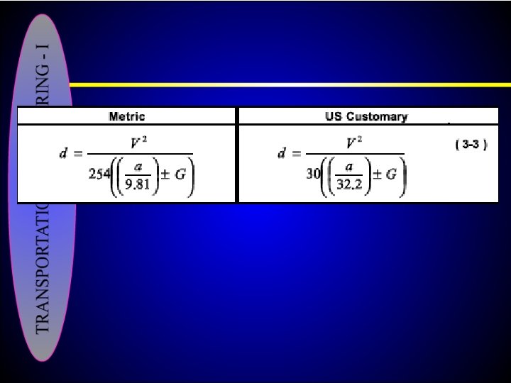
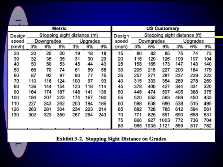
Effect of Grade on Stopping When a highway is on a grade, the equation for braking distance should be modified as follows: Eq 3 Where G is grade or longitudinal slope of the highway divided by 100.

Stopping sight distances calculated as based on Equation (2)

However, at the end of long down grades where truck speeds approach or exceed passenger car speeds, it is desirable to provide distances greater than those recommended in Exhibit 1 or even those calculated based on Equation (3). It is easy to see that under these circumstances higher eye position of the truck driver can be of little advantage.

Discussion The driver's reaction time, the condition of the road pavement, vehicle braking system, and the prevailing weather all play a significant role in this problem.

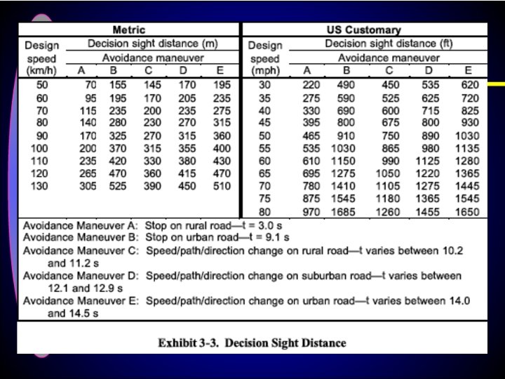
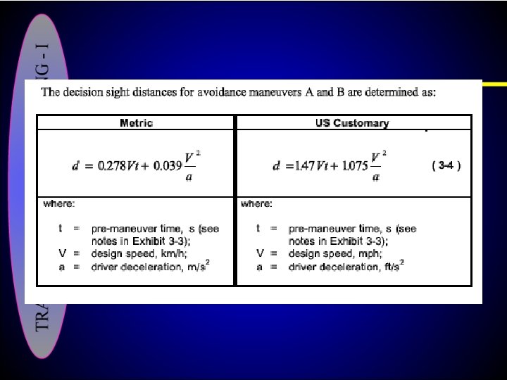
Decision Sight Distance Although stopping sight distances are generally sufficient to allow competent and alert drivers to stop their vehicles under ordinary circumstances, these distances are insufficient when information is difficult to perceive. When a driver is required to detect an unexpected or otherwise difficult to perceive information source, a decision sight distance should be provided.

Interchanges and inter sections, changes in cross section such as toll plazas and lane drops, and areas with "visual noise" are examples where drivers need decision sight distances. Exhibit 3 3, provides values used by designers for appropriate sight distances.

These values are applicable to most situations and have been developed from empirical data. Because of additional maneuvering space needed for safety, it is recommended that decision sight distances be provided at critical locations or critical decision points may be moved to where adequate distances are available.

If it is not practical to provide decision sight distance because of horizontal or vertical curvature or if relocation of decision points is not practical, special attention should be given to the use of suitable traffic control devices for providing advance warning of the conditions that are likely to be encountered.

Distances in Exhibit 3 3 for avoidance maneuvers A and B are calculated as based on Equation (2); however, with modified driver reaction time as stated in the notes for Exhibit 3 3. Decision sight distances for maneuvers C, D, and E are calculated from either 0. 278 Vt or 1. 47 V t, with t, modified as in the notes.

In computing and measuring stopping sight distances, driver's eye height is estimated as 1080 mm (3. 5 ft) and the height of the dangerous object seen by the driver is 600 mm (2. 0 ft), which represents the height of tail lights of a passenger car.

Stopping Sight Distance on plane Road Braking Distance on sloping Road Decision Distance

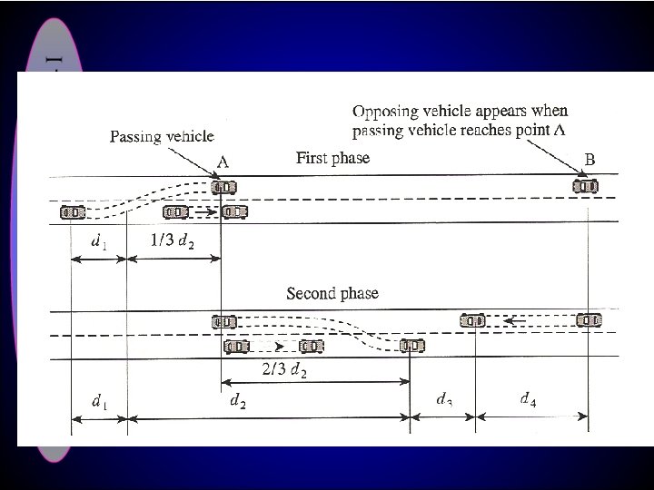
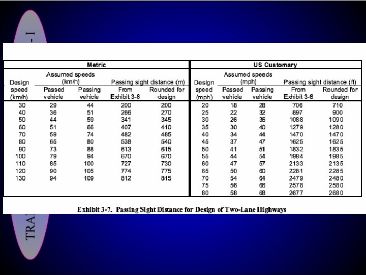
Passing Sight Distance for Two Lane Highways On most two lane, two way highways, vehicles frequently overtake slower moving vehicles by using the lane meant for the opposing traffic. To complete the passing maneuver safely, the driver should be able to see a sufficient distance ahead. Passing sight distance is determined on the basis that a driver wishes to pass a single vehicle, although multiple vehicle passing is permissible.

Based on observed traffic behavior, the following assumptions are made: 1. The overtaken vehicle travels at a uniform speed. 2. The passing vehicle has reduced speed and trails the overtaken vehicle as it enters a passing section. 3. The passing driver requires a short period of time to perceive the clear passing section, when reached, and to start maneuvering.

4)The passing vehicle accelerates during the maneuver, during the occupancy of the right lane, at about 15 km/h (10 mph) higher than the overtaken vehicle. 5)There is a suitable clearance length between the passing vehicle and the oncoming vehicle upon completion of the maneuver. The minimum passing sight distance for two lane highways is determined as the sum of the four distances shown in Figures on next slides.

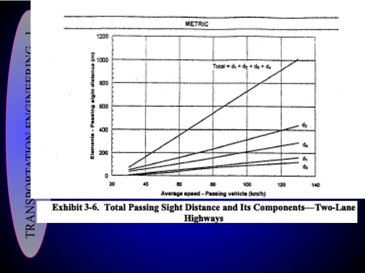
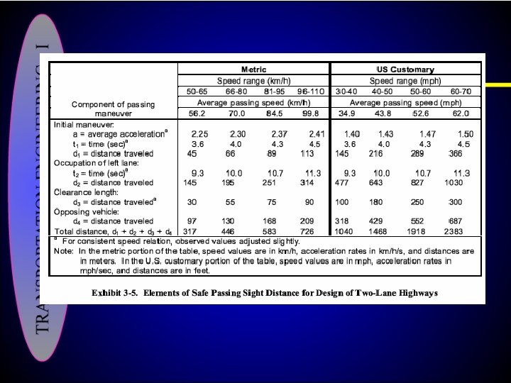
Safe passing sight distances for various speed ranges determined from distance and time values observed in the field are summarized in Exhibit 3 5

Initial maneuver distance d 1 The distance d 1 traveled during the initial maneuver period is computed with the following equation:

Distance while passing vehicle occupies left lane (d 2). Passing vehicles were found in the study to occupy the left lane from 9. 3 to 10. 4 s. The distance d 2 traveled in the left lane by the passing vehicle is computed with the following equation:

Clearance length (d 3). The clearance length between the opposing and passing vehicles at the end of the passing maneuvers was found in the passing study to vary from 30 to 75 m [100 to 250 ft].

Distance traversed by an opposing vehicle (d 4) The opposing vehicle is assumed to be traveling at the same speed as the passing vehicle, so

Initial maneuver distance d 1 Distance while passing vehicle occupies left lane (d 2). Clearance length (d 3). The clearance length between the opposing and passing vehicles at the end of the passing maneuvers was found in the passing study to vary from 30 to 75 m [100 to 250 ft]. Distance traversed by an opposing vehicle (d 4) d 4=2/3 d 2

Estimation of Velocity of a Vehicle just Before it is Involved in an accident Some times it is necessary to determine the velocity of a vehicle just before it is involved in an accident. Following steps are involved: 1) Estimate length of skid marks for all the four tires of the vehicle and take the average length. This is equal to breaking distance.

2)Find out “f” by performing trial runs under same environment /weather conditions and using a vehicle having similar conditions of tyres. Vehicle is driven at a known speed and breaking distance is measured. 3)The unknown speed is than determined using the braking formula.

Horizontal Alignment • Along circular path, vehicle undergoes centripetal acceleration towards center of curvature (lateral acceleration). • Balanced by superelevation and weight of vehicle (friction between tire and roadway). • Design based on appropriate relationship between design speed and curvature and their relationship with side friction and super elevation.

Vehicle Cornering Fcp Rv Fcn Fc e W Ff Wn Wp Ff 1 ft

• Figure illustrates the forces acting on a vehicle during cornering. In this figure, is the angle of inclination, W is the weight of the vehicle in pounds with Wn and Wp being the weight normal and parallel to the roadway surface respectively.

• Ff is the side frictional force, Fc is the centrifugal force with Fcp being the centrifugal force acting parallel to the roadway surface, Fcn is the centrifugal force acting normal to the roadway surface, and Rv is the radius defined to the vehicle’s traveled path in ft.

• Some basic horizontal curve relationships can be derived by summing forces parallel to the roadway surface. Wp + Ff = Fcp • From basic physics this equation can be written as

• Where fs is the coefficient of side friction, g is the gravitational constant and V is the vehicle speed (in ft per second). • Dividing both the sides of the equation by W cos ;

• The term tan is referred to as the super elevation of the curve and is denoted by ‘e’. • Super elevation is tilting the roadway to help offset centripetal forces developed as the vehicle goes around a curve. • The term ‘fs’ is conservatively set equal to zero for practical applications due to small values that ‘fs’ and ‘ ’ typically assume.

• With e = tan , equation can be rearranged as • Here Rv in meters • V speed in Km/hr • G=9. 8 m/sec 2 • e = coefficient of friction For Imperial units: V in mph And Rv in feet

Superelevation ew

Superelevation ie

Superelevation

Superelevation w P

Superelevation w

Superelevation

Superelevation w P

Superelevation . 5% V

Superelevation ie

Superelevation i

Super elevation

Superelevation w P

Superelevation w P

Superelevation w P

Superelevation w P

Superelevation w P

Superelevation w P

Superelevation w P

Superelevation w P

Superelevation w P

Superelevation w P

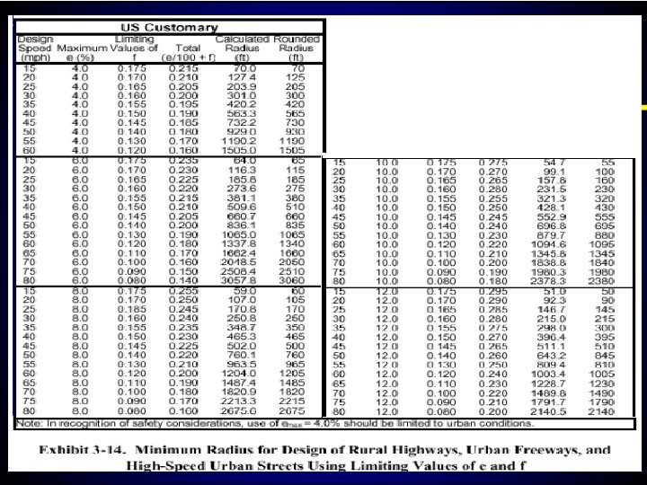
• In actual design of a horizontal curve, the engineer must select appropriate values of e and fs. • Super elevation value ‘e’ is critical since – high rates of super elevation cause vehicle steering problems at exits on horizontal curves – and in cold climates, ice on road ways can reduce fs and vehicles are forced inwardly off the curve by gravitational forces. • Values of ‘e’ and ‘fs’ can be obtained from AASHTO standards.

Horizontal Curve Fundamentals • For connecting straight tangent sections of roadway with a curve, several options are available. • The most obvious is the simple curve, which is just a standard curve with a single, constant radius. • Other options include; – compound curve, which consists of two or more simple curves in succession , – and spiral curves which are continuously changing radius curves.

Basic Geometry Tangent Horizontal Curve Tangent

Tangent Vs. Horizontal Curve • Predicting speeds for tangent and horizontal segments is different • May actually be easier to predict speeds on curves than tangents – Speeds on curves are restricted to a few well defined variables (e. g. radius, superelevation) – Speeds on tangents are not as restricted by design variables (e. g. driver attitude)

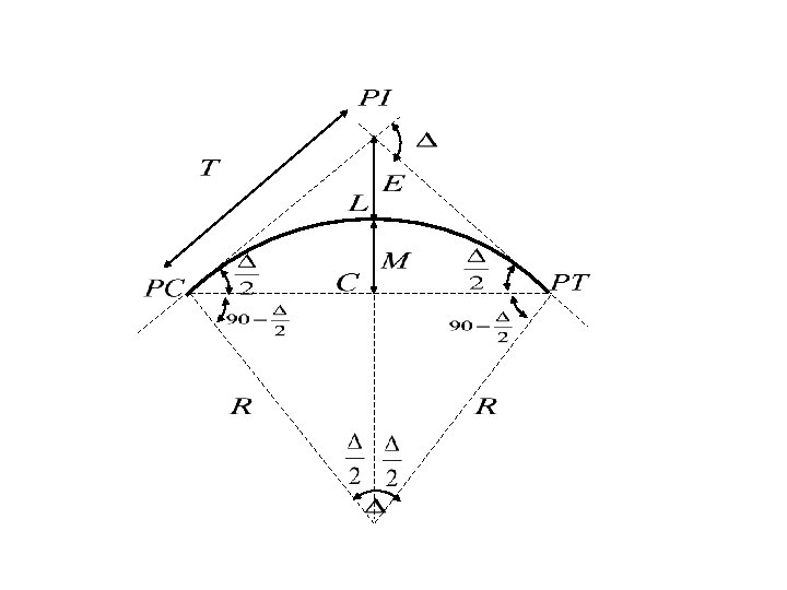
Elements of Horizontal Curves PI E T M L PC PT R R

• Figure shows the basic elements of a simple horizontal curve. In this figure – R is the radius (measured to center line of the road) – PC is the beginning point of horizontal curve – T is tangent length – PI is tangent intersection – is the central angle of the curve – PT is end point of curve – M is the middle ordinate – E is the external distance – L is the length of the curve

Degree of Curve • It is the angle subtended by a 100 ft arc along the horizontal curve. • Is a measure of the sharpness of curve and is frequently used instead of the radius in the actual construction of horizontal curve. • The degree of curve is directly related to the radius of the horizontal curve by

• A geometric and trigonometric analysis of figure, reveals the following relationships PI E T M L PC PT R R

Stopping Sight Distance and Horizontal Curve Design SSD Ms Sight Obstruction Highway Centerline Rv Critical inside lane s

• Adequate stopping sight distance must also be provided in the design of horizontal curves. • Sight distance restrictions on horizontal curves occur when obstructions are present. • Such obstructions are frequently encountered in highway design due to the cost of right of way acquisition and/or cost of moving earthen materials.

• When such an obstruction exists, the stopping sight distance is measured along the horizontal curve from the center of the traveled lane. • For a specified stopping sight distance, some distance, Ms, must be visually cleared, so that the line of sight is such that sufficient stopping sight distance is available.

• Equations for computing SSD relationships for horizontal curves can be derived by first determining the central angle, s, for an arc equal to the required stopping sight distance.

• Assuming that the length of the horizontal curve exceeds the required SSD, we have Combining the above equation with following we get;

• Rv is the radius to the vehicle’s traveled path, which is also assumed to be the location of the driver’s eye for sight distance, and is again taken as the radius to the middle of the innermost lane, • and s is the angle subtended by an arc equal to SSD in length.

• By substituting equation for s in equation of middle ordinate, we get the following equation for middle ordinate; • Where Ms is the middle ordinate necessary to provide adequate stopping sight distance. Solving further we get;

Max e • Controlled by 4 factors: – Climate conditions (amount of ice and snow) – Terrain (flat, rolling, mountainous) – Frequency of slow moving vehicles which influenced by high superelevation rates – Highest in common use = 10%, 12% with no ice and snow on low volume gravel surfaced roads – 8% is logical maximum to minimized slipping by stopped vehicles

Example A curving roadway has a design speed of 110 km/hr. At one horizontal curve, the Super elevation has been set at 6. 0% and the coefficient of side friction is found to be 0. 10. Determine the minimum radius of the curve that will provide safe R = 1102/9. 8(0. 10+0. 06) = 595 meters

Radius Calculation (Example) Design radius example: assume a maximum e of 8% and design speed of 60 mph, what is the minimum radius? fmax = 0. 12 (from Green Book) Rmin = _____602________ 15(0. 08 + 0. 12) Rmin = 1200 feet

Radius Calculation (Example) For emax = 4%? Rmin = _____602_____ 15(0. 04 + 0. 12) Rmin = 1, 500 feet

Sight Distance Example A horizontal curve with R = 800 ft is part of a 2 lane highway with a posted speed limit of 35 mph. What is the minimum distance that a large billboard can be placed from the centerline of the inside lane of the curve without reducing required SSD? Assume b/r =2. 5 sec and a = 11. 2 ft/sec 2 SSD is given as SSD = 1. 47 vt + _____v 2____ 30(__a___ G) 32. 2 SSD = 1. 47(35 mph)(2. 5 sec) + _____(35 mph)2____ 30(__11. 2___ 0) 32. 2 = 246 feet

Sight Distance Example m = R(1 – cos [28. 65 S]) R m = 800 (1 – cos [28. 65 {246}]) = 9. 43 feet 800 (in radians not degrees)

Horizontal Curve Example • Deflection angle of a 4º curve is 55º 25’, PC at station 238 + 44. 75. Find length of curve, T, and station of PC. • D = 4º • = 55º 25’ = 55. 417º • D = _5729. 58_ R = _5729. 58_ = 1, 432. 4 ft R 4

Horizontal Curve Example • D = 4º • = 55. 417º • R = 1, 432. 4 ft • L = 2 R = 2 (1, 432. 4 ft)(55. 417º) = 1385. 42 ft 360

Horizontal Curve Example • • D = 4º = 55. 417º R = 1, 432. 4 ft L = 1385. 42 ft • T = R tan = 1, 432. 4 ft tan (55. 417) = 752. 29 ft 2 2

Stationing Example Stationing goes around horizontal curve. For previous example, what is station of PT? PC = 238 + 44. 75 L = 1385. 42 ft = 13 + 85. 42 Station at PT = (238 + 44. 75) + (13 + 85. 42) = 252 + 30. 17

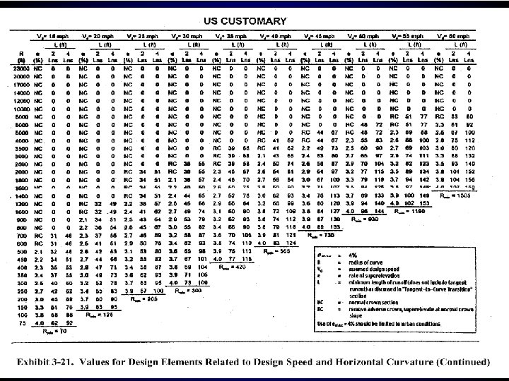
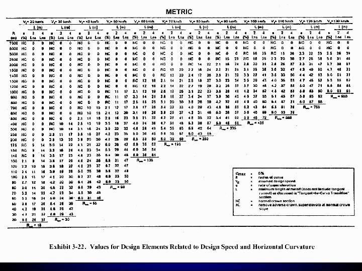
Suggested Steps on Horizontal Design 1. Select tangents, PIs, and general curves make sure you meet minimum radii 2. Select specific curve radii/spiral and calculate important points (see lab) using formula or table (those needed for design, plans, and lab requirements) 3. Station alignment (as curves are encountered) 4. Determine super and runoff for curves and put in table (see next lecture for def. ) 5. Add information to plans

Geometric Design – Horizontal Alignment (1) • Horizontal curve – Plan view, profile, staking, stationing – type of horizontal curves – Characteristics of simple circular curve • Stopping sight distance on horizontal curves • Spiral curve Lecture 8

Plan view and profile plan profile

Surveying and Stationing • Staking: route surveyors define the geometry of a highway by “staking” out the horizontal and vertical position of the route and by marking of the cross-section at intervals of 100 ft. • Station: Start from an origin by stationing 0, regular stations are established every 100 ft. , and numbered 0+00, 12 + 00 (=1200 ft), 20 + 45 (2000 ft + 45) etc.

Horizontal Curve Types

Curve Types 1. Simple curves with spirals 2. Broken Back – two curves same direction (avoid) 3. Compound curves: multiple curves connected directly together (use with caution) go from large radii to smaller radii and have R(large) < 1. 5 R(small) 4. Reverse curves – two curves, opposite direction (require separation typically for superelevation attainment)

1. Simple Curve Circular arc R Straight road sections

2. Compound Curve Circular arcs R 1 Straight road sections R 2

3. Broken Back Curve Circular arc Straight road sections

4. Reverse Curve Circular arcs Straight road sections

5. Spiral R = Rn R= Straight road section

Angle measurement (a) degree (b) Radian

As the subtended arc is proportional to the radius of the circle, then the radian measure of the angle Is the ratio of the length of the subtended arc to the radius of the circle

• • • • Define horizontal Curve: Circular Horizontal Curve Definitions Radius, usually measured to the centerline of the road, in ft. = Central angle of the curve in degrees PC = point of curve (the beginning point of the horizontal curve) PI = point of tangent intersection PT = Point of tangent (the ending point of the horizontal curve) T = tangent length in ft. M = middle ordinate from middle point of cord to middle point of curve in ft. E = External distance in ft. L = length of curve D = Degree of curvature (the angle subtended by a 100 -ft arc* along the horizontal curve) C = chord length from PC to PT * Note: use chord in practice

Key measures of the curve Note converts from radians to degrees

Example: A horizontal curve is designed with a 2000 -ft radius, the curve has a tangent length of 400 ft and The PI is at station 103 + 00, determine the stationing of the PT. Solution:

Sight Distance on Horizontal Curve: Minimum sight distance (for safety) should be equal to the safe stopping distance Sight Distance Highway Centerline M PC PT Line of sight Sight Obstruction Centerline of inside lane R R

To provide minimum sight distance: Or, by the degree of curvature, D Try yourself Where, ds = safe stopping distance, ft. and, v = design speed, mi/h t = reaction time, secs G = grade, % ds = stopping distance, in ft. a =deceleration rate, 11. 2 ft/s 2, recommended by Green Book

Example: A 6 degree curve (measured at the centerline of the inside lane) is being designed for a highway with a design speed of 70 mi/hr. , the grade is level, the driver reaction time is taken as 2. 5 s (ASSHTO’s standard value). What is the closest place that a roadside object (trees etc) can be Placed? Solution: The closest place of a object is given by:

Spiral Curve: Spiral curves are curves with a continuously changing radii, they are sometimes used on high-speed roadways with sharp horizontal curves and are sometimes used to gradually introduce the super elevation of an upcoming horizontal curve