TRANSMISSION OF INFORMATION Halim Yanikomeroglu and David Falconer

TRANSMISSION OF INFORMATION Halim Yanikomeroglu and David Falconer Systems and Computer Engineering Carleton University 1

Topics to be Covered l Analog and digital signals l Power spectral density and bandwidth l Analog to digital conversion (ADC): l PCM (pulse code modulation) l Digital transmission 2

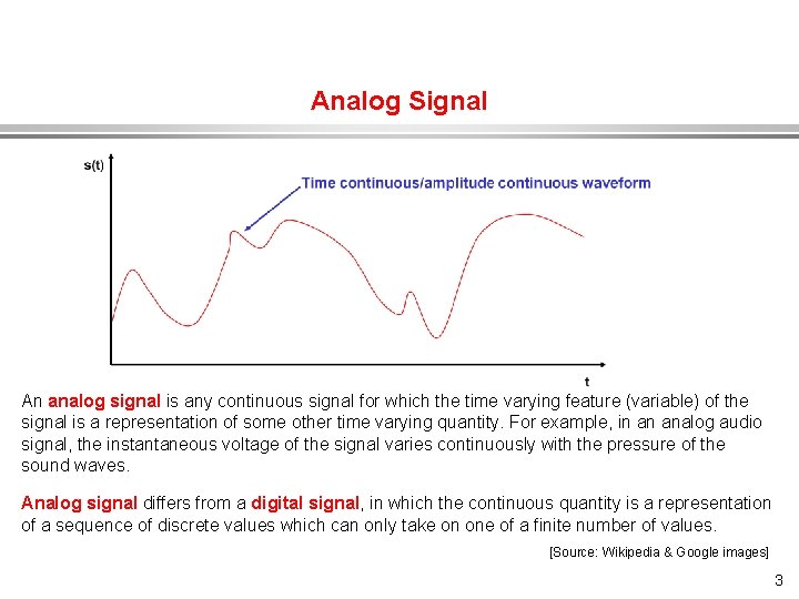
Analog Signal An analog signal is any continuous signal for which the time varying feature (variable) of the signal is a representation of some other time varying quantity. For example, in an analog audio signal, the instantaneous voltage of the signal varies continuously with the pressure of the sound waves. Analog signal differs from a digital signal, in which the continuous quantity is a representation of a sequence of discrete values which can only take on one of a finite number of values. [Source: Wikipedia & Google images] 3

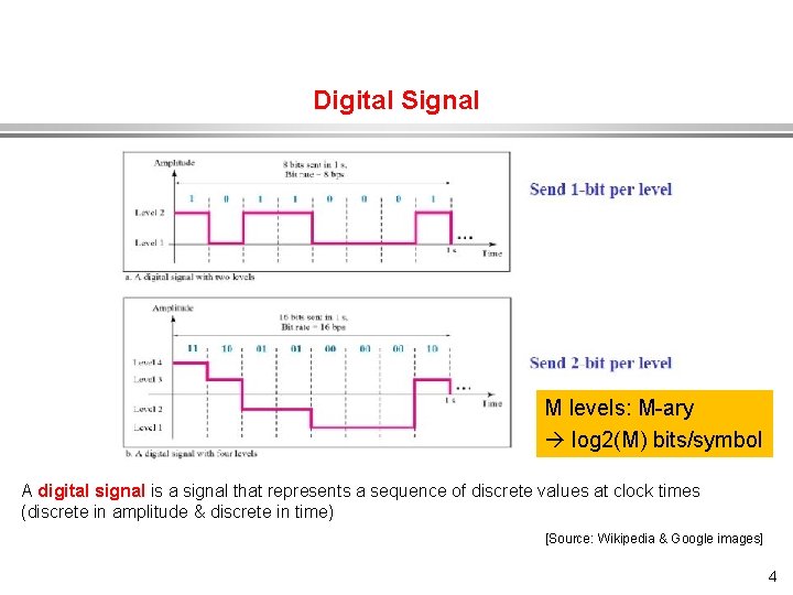
Digital Signal M levels: M-ary log 2(M) bits/symbol A digital signal is a signal that represents a sequence of discrete values at clock times (discrete in amplitude & discrete in time) [Source: Wikipedia & Google images] 4

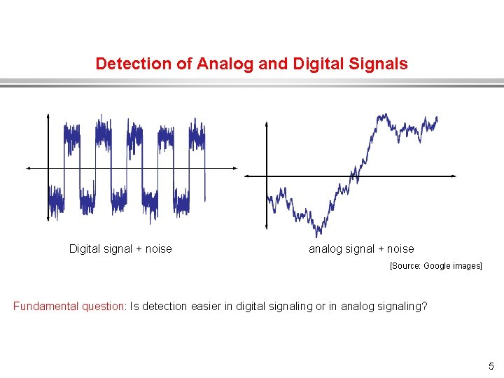
Detection of Analog and Digital Signals Digital signal + noise analog signal + noise [Source: Google images] Fundamental question: Is detection easier in digital signaling or in analog signaling? 5

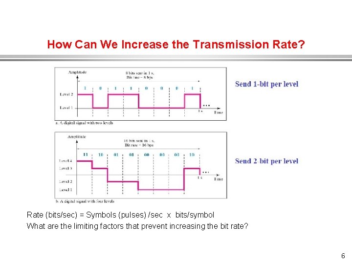
How Can We Increase the Transmission Rate? Rate (bits/sec) = Symbols (pulses) /sec x bits/symbol What are the limiting factors that prevent increasing the bit rate? 6

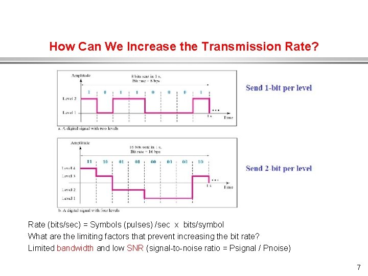
How Can We Increase the Transmission Rate? Rate (bits/sec) = Symbols (pulses) /sec x bits/symbol What are the limiting factors that prevent increasing the bit rate? Limited bandwidth and low SNR (signal-to-noise ratio = Psignal / Pnoise) 7

Digital and Analog Signals Some signals (like speech and video) are inherently analog; some (like computer data) are inherently digital. However, both analog and digital signals can be represented and transmitted digitally. Advantages of digital: » » » Reduced sensitivity to line noise, temp. drift, etc. Low cost digital VLSI for switching and transmission. Lower maintenance costs than analog. Uniformity in carrying voice, SMS, email, data, video, etc. (a bit is a bit). Better encryption. 8

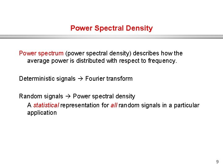
Power Spectral Density Power spectrum (power spectral density) describes how the average power is distributed with respect to frequency. Deterministic signals Fourier transform Random signals Power spectral density A statistical representation for all random signals in a particular application 9

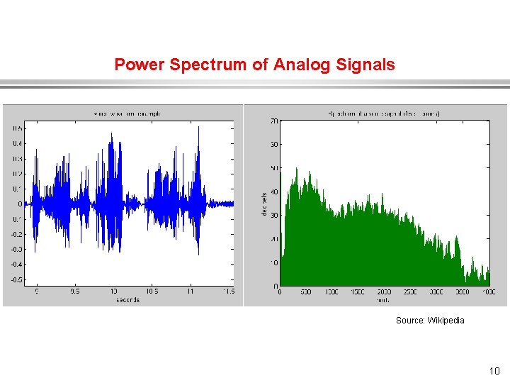
Power Spectrum of Analog Signals Source: Wikipedia 10

Power Spectrum of Analog Signals Analog (continuous-time, continuous-amplitude) signals (like speech) have a certain bandwidth. Their power spectrum (power spectral density) describes how their average power is distributed with respect to frequency. Power spectral density (watts/Hz) Watts per Hz = Joules “High-fidelity speech Bandwidth Telephone speech (limited by filtering) 0 1 2 3 4 5 6 7. . 11

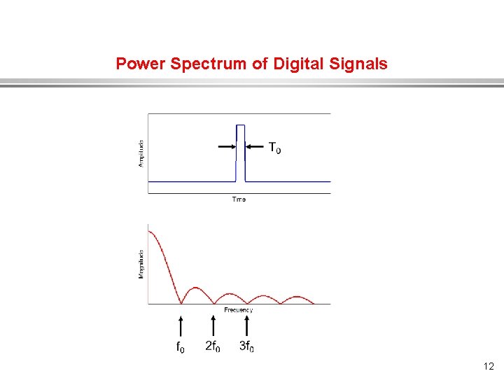
Power Spectrum of Digital Signals 12

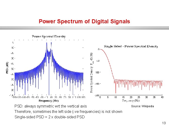
Power Spectrum of Digital Signals PSD: always symmetric wrt the vertical axis Therefore, sometimes the left side (-ve frequencies) is not shown Single-sided PSD = 2 x double-sided PSD Source: Wikipedia 13

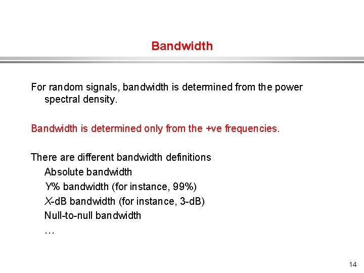
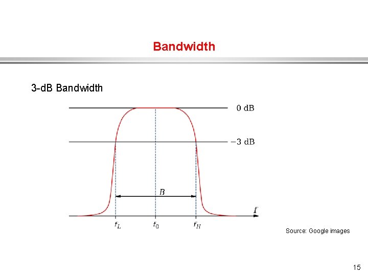
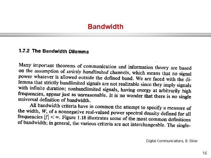
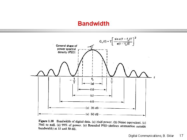
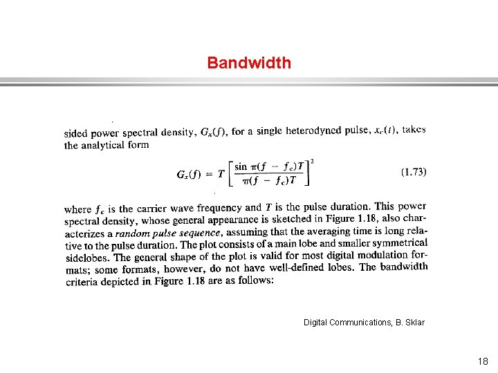
Bandwidth For random signals, bandwidth is determined from the power spectral density. Bandwidth is determined only from the +ve frequencies. There are different bandwidth definitions Absolute bandwidth Y% bandwidth (for instance, 99%) X-d. B bandwidth (for instance, 3 -d. B) Null-to-null bandwidth … 14

Bandwidth 3 -d. B Bandwidth Source: Google images 15

Bandwidth Digital Communications, B. Sklar 16

Bandwidth Digital Communications, B. Sklar 17

Bandwidth Digital Communications, B. Sklar 18

Bandwidth Digital Communications, B. Sklar 19

Analog to Digital Conversion (ADC) Convert the analog signal to digital format (“ 0”s and “ 1”s) as efficient as possible, and as accurately as possible. Efficiency: Less resources in storage and/or transmission (bandwidth, rate). Accuracy: High fidelity. 20

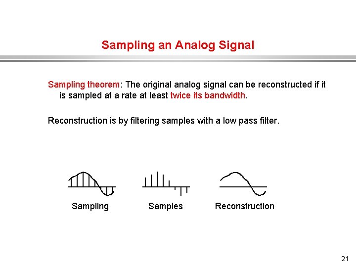
Sampling an Analog Signal Sampling theorem: The original analog signal can be reconstructed if it is sampled at a rate at least twice its bandwidth. Reconstruction is by filtering samples with a low pass filter. Sampling Samples Reconstruction 21

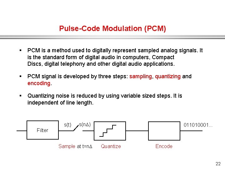
Pulse-Code Modulation (PCM) § PCM is a method used to digitally represent sampled analog signals. It is the standard form of digital audio in computers, Compact Discs, digital telephony and other digital audio applications. § PCM signal is developed by three steps: sampling, quantizing and encoding. § Quantizing noise is reduced by using variable sized steps. It is independent of line length. s(t) s(n ) Filter 011010001. . . Sample at t=n Quantize Encode 22

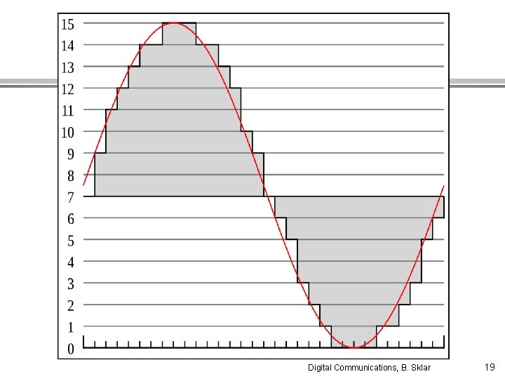
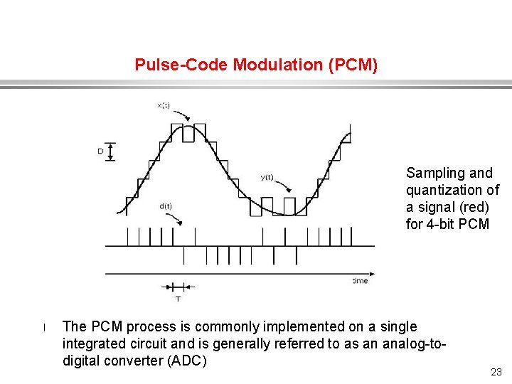
Pulse-Code Modulation (PCM) Sampling and quantization of a signal (red) for 4 -bit PCM l The PCM process is commonly implemented on a single integrated circuit and is generally referred to as an analog-todigital converter (ADC) 23

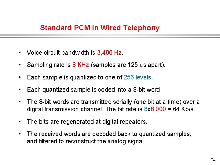
Standard PCM in Wired Telephony • Voice circuit bandwidth is 3, 400 Hz. • Sampling rate is 8 KHz (samples are 125 s apart). • Each sample is quantized to one of 256 levels. • Each quantized sample is coded into a 8 -bit word. • The 8 -bit words are transmitted serially (one bit at a time) over a digital transmission channel. The bit rate is 8 x 8, 000 = 64 Kb/s. • The bits are regenerated at digital repeaters. • The received words are decoded back to quantized samples, and filtered to reconstruct the analog signal. 24

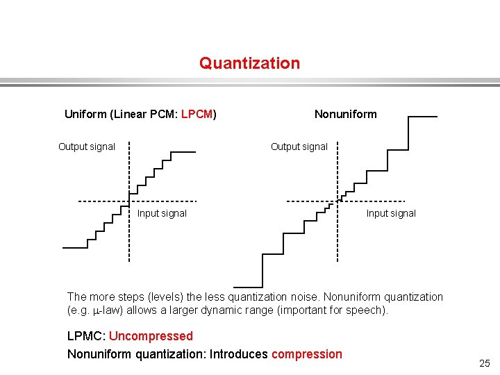
Quantization Uniform (Linear PCM: LPCM) Output signal Nonuniform Output signal Input signal The more steps (levels) the less quantization noise. Nonuniform quantization (e. g. -law) allows a larger dynamic range (important for speech). LPMC: Uncompressed Nonuniform quantization: Introduces compression 25

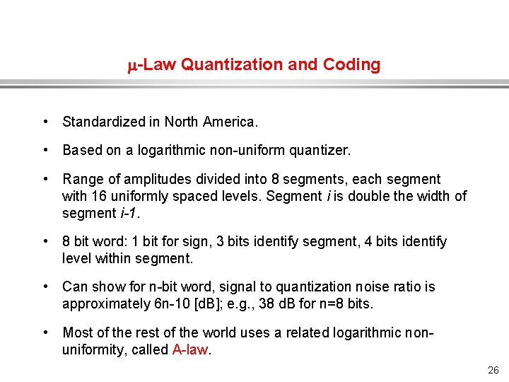
-Law Quantization and Coding • Standardized in North America. • Based on a logarithmic non-uniform quantizer. • Range of amplitudes divided into 8 segments, each segment with 16 uniformly spaced levels. Segment i is double the width of segment i-1. • 8 bit word: 1 bit for sign, 3 bits identify segment, 4 bits identify level within segment. • Can show for n-bit word, signal to quantization noise ratio is approximately 6 n-10 [d. B]; e. g. , 38 d. B for n=8 bits. • Most of the rest of the world uses a related logarithmic nonuniformity, called A-law. 26

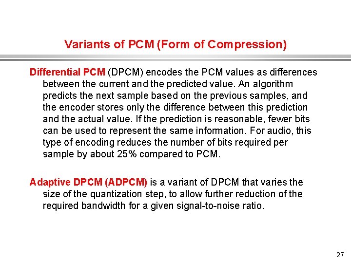
Variants of PCM (Form of Compression) Differential PCM (DPCM) encodes the PCM values as differences between the current and the predicted value. An algorithm predicts the next sample based on the previous samples, and the encoder stores only the difference between this prediction and the actual value. If the prediction is reasonable, fewer bits can be used to represent the same information. For audio, this type of encoding reduces the number of bits required per sample by about 25% compared to PCM. Adaptive DPCM (ADPCM) is a variant of DPCM that varies the size of the quantization step, to allow further reduction of the required bandwidth for a given signal-to-noise ratio. 27

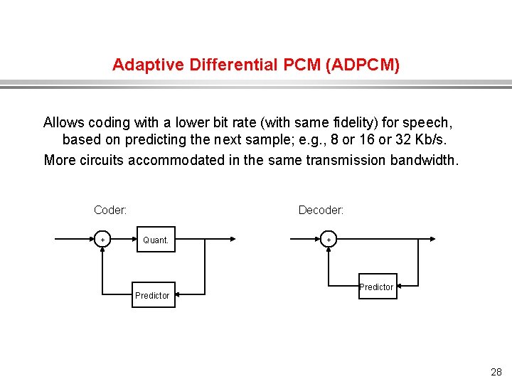
Adaptive Differential PCM (ADPCM) Allows coding with a lower bit rate (with same fidelity) for speech, based on predicting the next sample; e. g. , 8 or 16 or 32 Kb/s. More circuits accommodated in the same transmission bandwidth. Coder: + Decoder: Quant. Predictor + Predictor 28

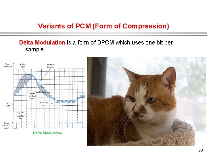
Variants of PCM (Form of Compression) Delta Modulation is a form of DPCM which uses one bit per sample. 29

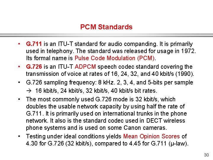
PCM Standards • G. 711 is an ITU-T standard for audio companding. It is primarily used in telephony. The standard was released for usage in 1972. Its formal name is Pulse Code Modulation (PCM). • G. 726 is an ITU-T ADPCM speech codec standard covering the transmission of voice at rates of 16, 24, 32, and 40 kbit/s (1990). • G. 726 sampling frequency: 8 k. Hz. 2, 3, 4, and 5 -bits per sample 16 kbit/s, 24 kbit/s, 32 kbit/s, 40 kbit/s bit rates. • The most commonly used G. 726 mode is 32 kbit/s, which doubles the usable network capacity by using half the rate of G. 711. It is primarily used on international trunks in the phone network. It also is the standard codec used in DECT wireless phone systems and is used on some Canon cameras. • Testing under ideal conditions yields Mean Opinion Scores of 4. 30 for G. 726 (32 kbit/s), compared to 4. 45 for G. 711 (µ-law). 30

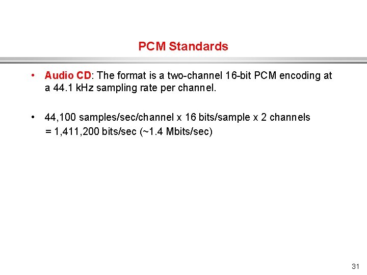
PCM Standards • Audio CD: The format is a two-channel 16 -bit PCM encoding at a 44. 1 k. Hz sampling rate per channel. • 44, 100 samples/sec/channel x 16 bits/sample x 2 channels = 1, 411, 200 bits/sec (~1. 4 Mbits/sec) 31

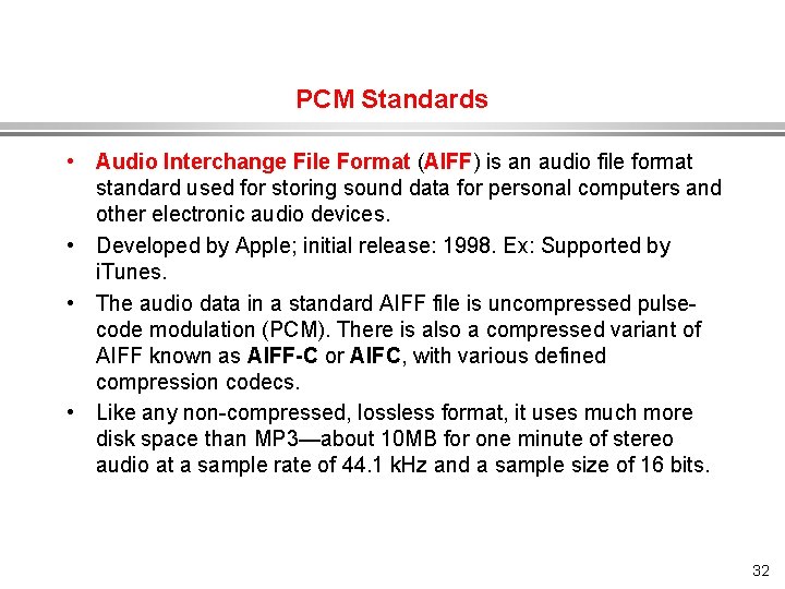
PCM Standards • Audio Interchange File Format (AIFF) is an audio file format standard used for storing sound data for personal computers and other electronic audio devices. • Developed by Apple; initial release: 1998. Ex: Supported by i. Tunes. • The audio data in a standard AIFF file is uncompressed pulsecode modulation (PCM). There is also a compressed variant of AIFF known as AIFF-C or AIFC, with various defined compression codecs. • Like any non-compressed, lossless format, it uses much more disk space than MP 3—about 10 MB for one minute of stereo audio at a sample rate of 44. 1 k. Hz and a sample size of 16 bits. 32

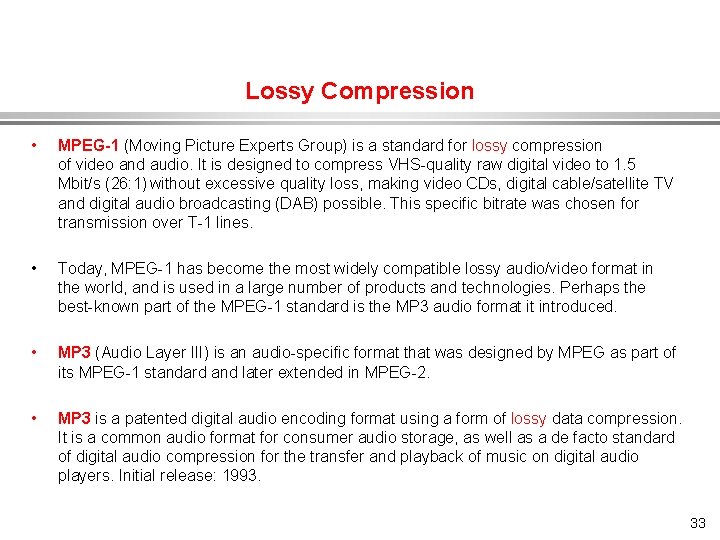
Lossy Compression • MPEG-1 (Moving Picture Experts Group) is a standard for lossy compression of video and audio. It is designed to compress VHS-quality raw digital video to 1. 5 Mbit/s (26: 1) without excessive quality loss, making video CDs, digital cable/satellite TV and digital audio broadcasting (DAB) possible. This specific bitrate was chosen for transmission over T-1 lines. • Today, MPEG-1 has become the most widely compatible lossy audio/video format in the world, and is used in a large number of products and technologies. Perhaps the best-known part of the MPEG-1 standard is the MP 3 audio format it introduced. • MP 3 (Audio Layer III) is an audio-specific format that was designed by MPEG as part of its MPEG-1 standard and later extended in MPEG-2. • MP 3 is a patented digital audio encoding format using a form of lossy data compression. It is a common audio format for consumer audio storage, as well as a de facto standard of digital audio compression for the transfer and playback of music on digital audio players. Initial release: 1993. 33

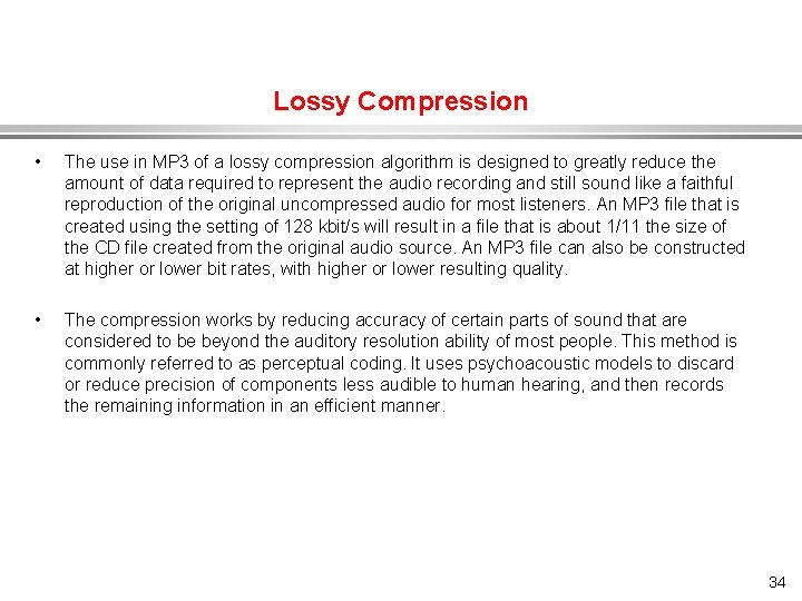
Lossy Compression • The use in MP 3 of a lossy compression algorithm is designed to greatly reduce the amount of data required to represent the audio recording and still sound like a faithful reproduction of the original uncompressed audio for most listeners. An MP 3 file that is created using the setting of 128 kbit/s will result in a file that is about 1/11 the size of the CD file created from the original audio source. An MP 3 file can also be constructed at higher or lower bit rates, with higher or lower resulting quality. • The compression works by reducing accuracy of certain parts of sound that are considered to be beyond the auditory resolution ability of most people. This method is commonly referred to as perceptual coding. It uses psychoacoustic models to discard or reduce precision of components less audible to human hearing, and then records the remaining information in an efficient manner. 34

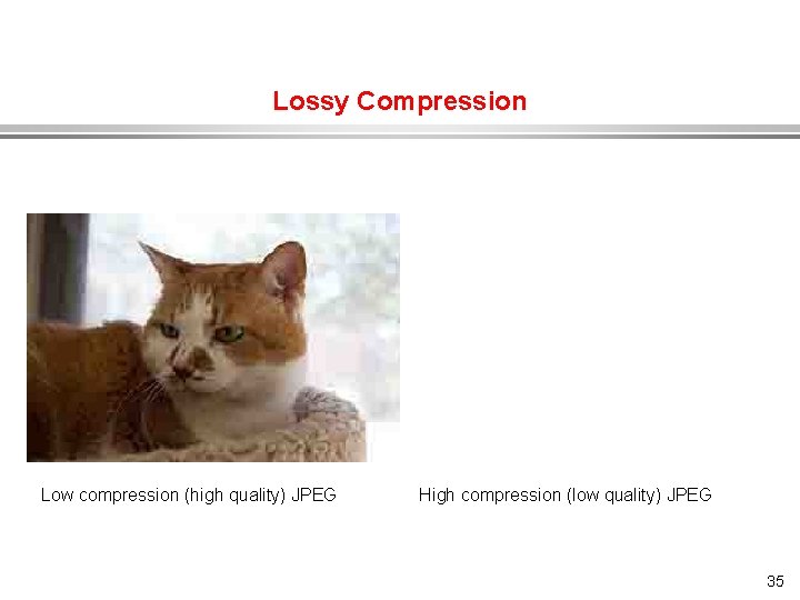
Lossy Compression Low compression (high quality) JPEG High compression (low quality) JPEG 35

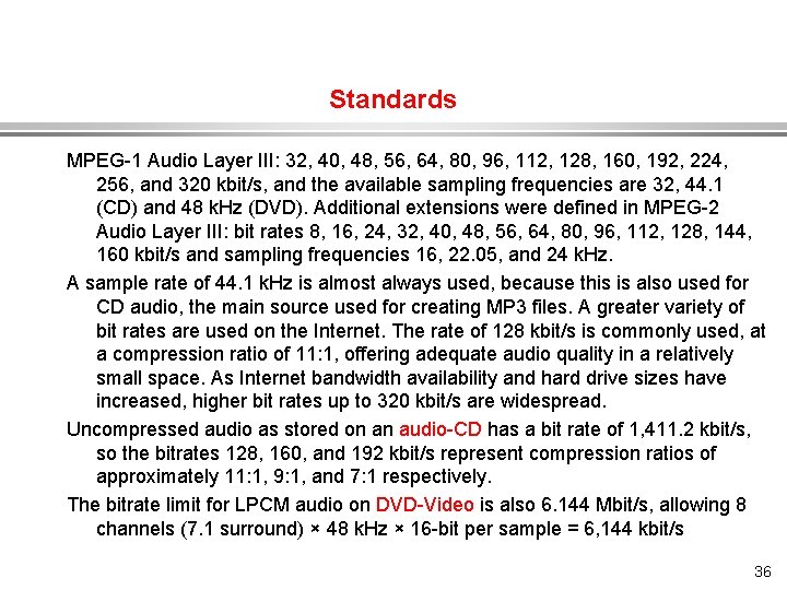
Standards MPEG-1 Audio Layer III: 32, 40, 48, 56, 64, 80, 96, 112, 128, 160, 192, 224, 256, and 320 kbit/s, and the available sampling frequencies are 32, 44. 1 (CD) and 48 k. Hz (DVD). Additional extensions were defined in MPEG-2 Audio Layer III: bit rates 8, 16, 24, 32, 40, 48, 56, 64, 80, 96, 112, 128, 144, 160 kbit/s and sampling frequencies 16, 22. 05, and 24 k. Hz. A sample rate of 44. 1 k. Hz is almost always used, because this is also used for CD audio, the main source used for creating MP 3 files. A greater variety of bit rates are used on the Internet. The rate of 128 kbit/s is commonly used, at a compression ratio of 11: 1, offering adequate audio quality in a relatively small space. As Internet bandwidth availability and hard drive sizes have increased, higher bit rates up to 320 kbit/s are widespread. Uncompressed audio as stored on an audio-CD has a bit rate of 1, 411. 2 kbit/s, so the bitrates 128, 160, and 192 kbit/s represent compression ratios of approximately 11: 1, 9: 1, and 7: 1 respectively. The bitrate limit for LPCM audio on DVD-Video is also 6. 144 Mbit/s, allowing 8 channels (7. 1 surround) × 48 k. Hz × 16 -bit per sample = 6, 144 kbit/s 36

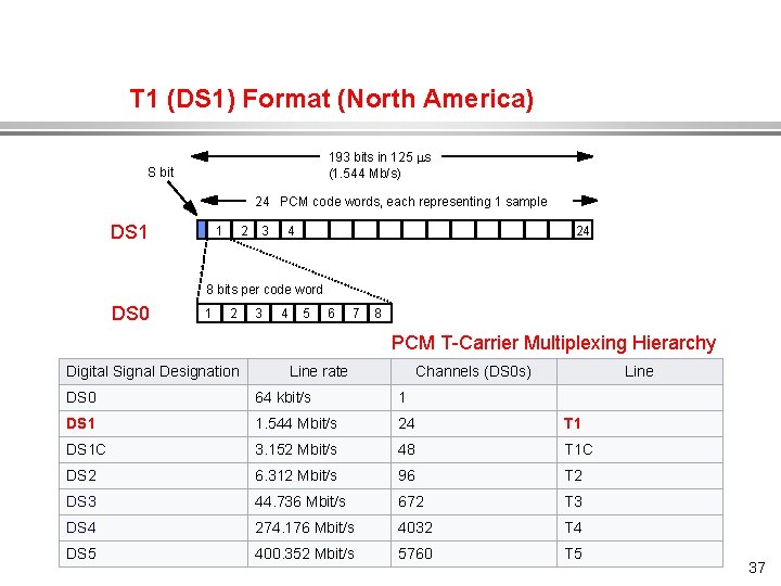
T 1 (DS 1) Format (North America) 193 bits in 125 s (1. 544 Mb/s) S bit 24 PCM code words, each representing 1 sample DS 1 1 2 3 4 24 8 bits per code word DS 0 1 2 3 4 5 6 7 8 PCM T-Carrier Multiplexing Hierarchy Digital Signal Designation Line rate Channels (DS 0 s) Line DS 0 64 kbit/s 1 DS 1 1. 544 Mbit/s 24 T 1 DS 1 C 3. 152 Mbit/s 48 T 1 C DS 2 6. 312 Mbit/s 96 T 2 DS 3 44. 736 Mbit/s 672 T 3 DS 4 274. 176 Mbit/s 4032 T 4 DS 5 400. 352 Mbit/s 5760 T 5 37

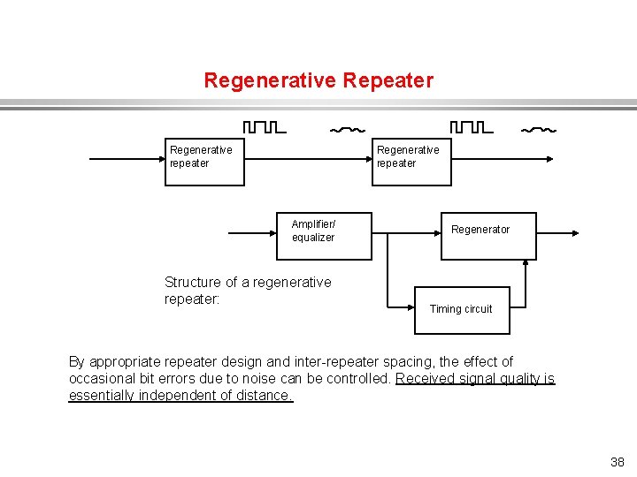
Regenerative Repeater Regenerative repeater Amplifier/ equalizer Structure of a regenerative repeater: Regenerator Timing circuit By appropriate repeater design and inter-repeater spacing, the effect of occasional bit errors due to noise can be controlled. Received signal quality is essentially independent of distance. 38

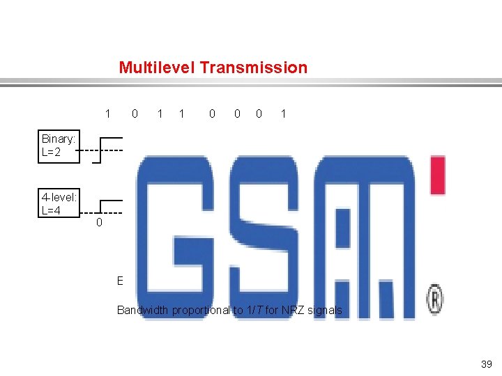
Multilevel Transmission 1 0 1 1 0 0 0 1 Binary: L=2 4 -level: L=4 0 T 2 T 3 T 4 T Bit rate = Bandwidth proportional to 1/T for NRZ signals 39

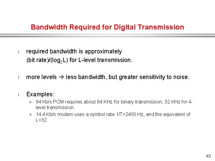
Bandwidth Required for Digital Transmission required bandwidth is approximately (bit rate)/(log 2 L) for L-level transmission. l l more levels less bandwidth, but greater sensitivity to noise. l Examples: » 64 Kb/s PCM requires about 64 KHz for binary transmission, 32 KHz for 4 level transmission. » 14. 4 Kb/s modem uses a symbol rate 1/T=2400 Hz, and the equivalent of L=32. 40

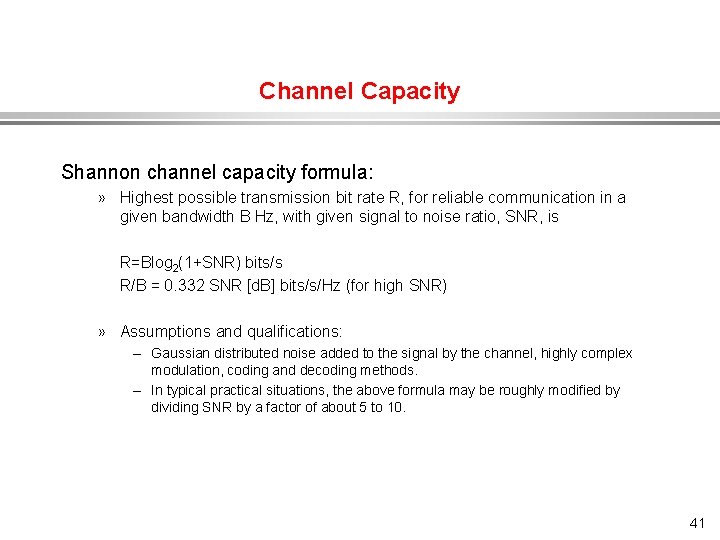
Channel Capacity Shannon channel capacity formula: » Highest possible transmission bit rate R, for reliable communication in a given bandwidth B Hz, with given signal to noise ratio, SNR, is R=Blog 2(1+SNR) bits/s R/B = 0. 332 SNR [d. B] bits/s/Hz (for high SNR) » Assumptions and qualifications: – Gaussian distributed noise added to the signal by the channel, highly complex modulation, coding and decoding methods. – In typical practical situations, the above formula may be roughly modified by dividing SNR by a factor of about 5 to 10. 41

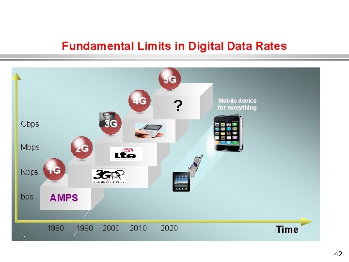
Fundamental Limits in Digital Data Rates 5 G 4 G 3 G Gbps Mbps Kbps ? Mobile device for everything 2 G 1 G AMPS 1980 1990 2000 2010 2020 l. Time 42

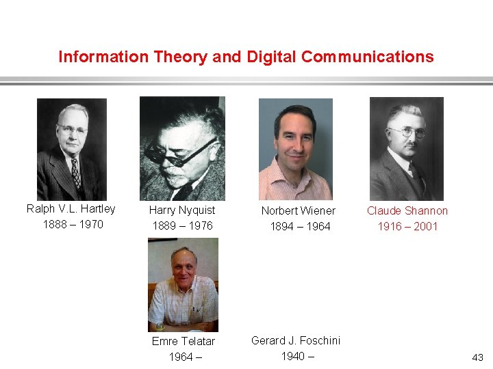
Information Theory and Digital Communications Ralph V. L. Hartley 1888 – 1970 Harry Nyquist 1889 – 1976 Norbert Wiener 1894 – 1964 Emre Telatar 1964 – Gerard J. Foschini 1940 – Claude Shannon 1916 – 2001 43

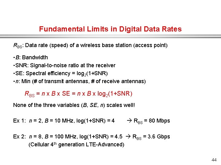
Fundamental Limits in Digital Data Rates RBS: Data rate (speed) of a wireless base station (access point) • B: Bandwidth • SNR: Signal-to-noise ratio at the receiver • SE: Spectral efficiency = log 2(1+SNR) • n: Min (# of transmit antennas, # of receive antennas) RBS = n x B x SE = n x B x log 2(1+SNR) None of the three variables (B, SE, n) scales well! Ex 1: n = 2, B = 10 MHz, log(1+SNR) = 4 RBS = 80 Mbps Ex 2: n = 8, B = 100 MHz, log(1+SNR) = 4. 5 RBS = 3. 6 Gbps (Cellular 4 th generation LTE-Advanced) 44

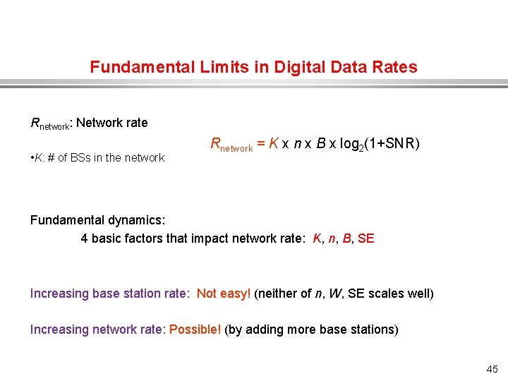
Fundamental Limits in Digital Data Rates Rnetwork: Network rate • K: # of BSs in the network Rnetwork = K x n x B x log 2(1+SNR) Fundamental dynamics: 4 basic factors that impact network rate: K, n, B, SE Increasing base station rate: Not easy! (neither of n, W, SE scales well) Increasing network rate: Possible! (by adding more base stations) 45

Summary l All information signals can be represented, switched, stored and transmitted digitally. l We have discussed PCM systems and their key elements: » » l sampling quantizing coding digital transmission We have discussed the related concepts of: » » power spectrum density bandwidth multiplexing channel capacity • We have discussed the fundamental enablers of transmission rate. 46