Transmission Lines Dr Sandra CruzPol ECE Dept UPRM

Transmission Lines Dr. Sandra Cruz-Pol ECE Dept. UPRM

Why is circuit theory different for high frequencies? . . Example A 40 -m long TL has Vg=15 Vrms, Zo=30+j 60 W, and VL=5 e-j 48 o Vrms. If the line is matched to the load and the generator, find: the sending-end Voltage Vin. Iin Zg Vg + Vin Zo=30+j 60 g=a +j b - VL - 40 m n + Answer: (we’ll see procedure later on) ZL

Voltage & Current are waves! Therefore their magnitude and phase change as they travel along space. n The higher the frequency, the faster it changes with space. n

Transmission Lines (TL) n TL have two conductors in parallel with a dielectric separating them n They transmit TEM waves inside the lines

Common Transmission Lines Two-wire (ribbon) Coaxial Microstrip Stripline (Triplate)

Other TL (higher order) [Chapter 11]

Fields inside the TL V proportional to E, n I proportional to H n

Transmission Lines TL parameters TL Equations Input Impedance, SWR, power Smith Chart Applications I. III. IV. V. ¨ ¨ ¨ VI. Quarter-wave transformer Slotted line Single stub Microstrips

Transmission Lines TL parameters TL Equations Input Impedance, SWR, power Smith Chart Applications I. III. IV. V. ¨ ¨ ¨ VI. Quarter-wave transformer Slotted line Single stub Microstrips

Distributed parameters The parameters that characterize the TL are given in terms of per length. n R = ohms/meter n L = Henries/ m n C = Farads/m n G = mhos/m

Common Transmission Lines R, L, G, and C depend on the particular transmission line structure and the material properties. R, L, G, and C can be calculated using fundamental EMAG techniques. Parameter R L G C Two-Wire Line Coaxial Line Parallel-Plate Line Unit

TL representation

Distributed line parameters Using KVL:

Distributed parameters n Taking the limit as Dz tends to 0 leads to n Similarly, applying KCL to the main node gives

Combine & we get …Wave equation n Using phasors n The two expressions reduce to Wave Equation for voltage

Transmission Lines TL parameters TL Equations Input Impedance, SWR, power Smith Chart Applications I. III. IV. V. ¨ ¨ ¨ VI. Quarter-wave transformer Slotted line Single stub Microstrips

TL Equations n Note that these are the wave eq. for voltage and current inside the lines. n The propagation constant is g and the wavelength and velocity are

Waves moves along line The general solution is n In time domain is n Similarly for current, I z

Characteristic Impedance of a Line, Zo n Is the ratio of positively traveling voltage wave to current wave at any point on the line z

Example: n n n An air filled planar line with w=30 cm, d=1. 2 cm, t=3 mm, sc=7 x 107 S/m. Find R, L, C, G for 500 MHz Answer d w

Exercise 11. 1 A transmission line operating at 500 MHz has Zo=80 W, a=0. 04 Np/m, b=1. 5 rad/m. Find the line parameters R, L, G, and C. n Answer: 3. 2 W/m, 38. 2 n. H/m, 0. 0005 S/m, 5. 97 p. F/m

Different cases of TL n Lossless n Distortionless Transmission line n Lossy Transmission line

Lossless Lines (R=0=G) Has perfect conductors and perfect dielectric medium between them. n Propagation: n Velocity: n Impedance

Distortionless line (R/L = G/C) Is one in which the attenuation is independent on frequency. n Propagation: n Velocity: n Impedance

Summary g = a + jb General Lossless Distortionless RC = GL Zo

Excersice 11. 2 n n A telephone line has R=30 W/km, L=100 m. H/km, G=0, and C= 20 m. F/km. At 1 k. Hz, obtain: the characteristic impedance of the line, the propagation constant, the phase velocity. Solution:

Define reflection coefficient at the load, GL

Terminated, Lossless TL Then, Similarly, The impedance anywhere along the line is given by The impedance at the load end, ZL, is given by

Terminated, Lossless TL Then, Conclusion: The reflection coefficient is a function of the load impedance and the characteristic impedance. Recall for the lossless case, Then

Example n n A generator with 10 Vrms and Rg=50, is connected to a 75 W load thru a 0. 8 l, 50 W-lossless line. Find VL

Terminated, Lossless TL It is customary to change to a new coordinate system, z = - l , at this point. -z z=-l Rewriting the expressions for voltage and current, we have Rearranging,

Transmission Lines TL parameters TL Equations Input Impedance, SWR, power Smith Chart Applications I. III. IV. V. ¨ ¨ ¨ VI. Quarter-wave transformer Slotted line Single stub Microstrips

Impedance (Lossy line) The impedance anywhere along the line is given by The reflection coefficient can be modified as follows Then, the impedance can be written as After some algebra, an alternative expression for the impedance is given by Conclusion: The load impedance is “transformed” as we move away from the load.

Impedance (Lossless line) The impedance anywhere along the line is given by The reflection coefficient can be modified as follows Then, the impedance can be written as After some algebra, an alternative expression for the impedance is given by

Exercise : using formulas n A 2 cm lossless TL has Vg=10 Vrms, Zg=60 W, ZL=100+j 80 W and Zo=40 W, l=10 cm. find: the input impedance Zin, the sending-end Voltage Vin, Iin Zg Vg + Vin Zo g=j b - VL - 2 cm Voltage Divider: + ZL

Transmission Lines TL parameters TL Equations Input Impedance, SWR, power Smith Chart Applications I. III. IV. V. ¨ ¨ ¨ VI. Quarter-wave transformer Slotted line Single stub Microstrips

SWR or VSWR or s Whenever there is a reflected wave, a standing wave will form out of the combination of incident and reflected waves. The (Voltage) Standing Wave Ratio - SWR (or VSWR) is defined as

Power n The average input power at a distance l from the load is given by n which can be reduced to n The first term is the incident power and the second is the reflected power. Maximum power is delivered to load if G=0

Three common Cases of line-load combinations: 1. Shorted Line (ZL=0) 2. Open-circuited Line (ZL=∞) 3. Matched Line (ZL = Zo)

Standing Waves -Shorted Line (ZL=0), we had Voltage maxima n So substituting in V(z) |V(z)| -z -l -l/2 -l/4 *Voltage minima occurs at same place that impedance has a minimum on the line

Standing Waves -Open Line (ZL=∞) , we had n So substituting in V(z) Voltage minima -z -l -l/2 |V(z)| -l/4

Standing Waves -Matched Line (ZL = Zo), we had n So substituting in V(z) |V(z)| -z -l -l/2 -l/4

Java applets http: //www. amanogawa. com/transmission. html n http: //physics. usask. ca/~hirose/ep 225/ n http: //www. educatorscorner. com/index. cgi ? CONTENT_ID=2483 n

Transmission Lines TL parameters TL Equations Input Impedance, SWR, power Smith Chart Applications I. III. IV. V. ¨ ¨ ¨ VI. Quarter-wave transformer Slotted line Single stub Microstrips

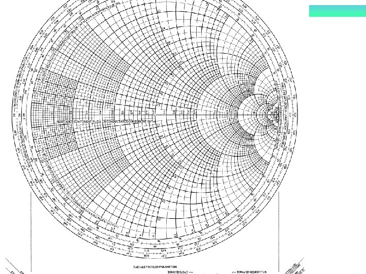
The Smith Chart

Smith Chart Commonly used as graphical representation of a TL. n Used in hi-tech equipment for design and testing of microwave circuits n One turn (360 o) around the SC = to l/2 n

Network Analyzer What can be seen on the screen?

Smith Chart n Suppose you use as coordinates the reflection coefficient real and imaginary parts. Gi and define the normalized ZL: |G| Gr

Now relating to z=r+jx n After some algebra, we obtain two eqs. Circles of r Circles of x n Similar to general equation of a circle of radius a, center at (h, k)

Examples of circles of r and x Circles of r Circles of x

Examples of circles of r and x Circles of r Circles of x

The joy of the SC Numerically s = r on the +axis of Gr in the SC Proof: n

Fun facts about the Smith Chart n A lossless TL is represented as a circle of constant radius, |G|, or constant s To generator n Moving along the line from the load toward the generator, the phase decrease, therefore, in the SC equals to moves clockwisely.

Fun facts about the Smith Chart n One turn (360 o) around the SC = to l/2 because in the formula below, if you substitute length for halfwavelength, the phase changes by 2 p, which is one turn. n Find the point in the SC where G=+1, -1, j, -j, 0, 0. 5 What is r and x for each case? n

Fun facts : Admittance in the SC n The admittance, y=YL/Yo where Yo=1/Zo, can be found by moving ½ turn (l/4) on the TL circle

Fun facts about the Smith Chart n n The Gr +axis, where r > 0 corresponds to Vmax The Gr -axis, where r < 0 corresponds to Vmin Vmax (Maximum impedance)

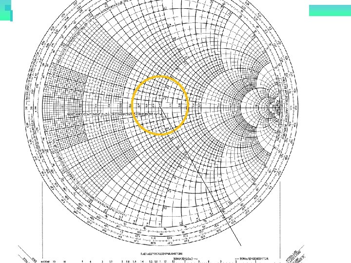
Exercise: using S. C. n A 2 cm lossless TL has Vg=10 Vrms, Zg=60 W, ZL=100+j 80 W and Zo=40 W, l=10 cm. find: the input impedance Zin, the sending-end Voltage Vin, Iin Zg Vg + Vin Zo g=j b - + VL - 2 cm n n n Load is at. 2179 l @ S. C. Move. 2 l and arrive to. 4179 l Read Voltage Divider: ZL

z. L zin 0. 2 l

Exercise: cont…. using S. C. n A 2 cm lossless TL has Vg=10 Vrms, Zg=60 W, ZL=100+j 80 W and Zo=40 W, l=10 cm. find: the input impedance Zin, the sending-end Voltage Vin, Iin Zg Vg + Vin Zo g=j b - + VL ZL - 2 cm n n Distance from the load (. 2179 l) to the nearest minimum & max Move to horizontal axis toward the generator and arrive to. 5 l (Vmax) and to. 25 l for the Vmin. Distance to min=. 5 -. 2179=. 282 l Distance to 2 st voltage maximum is. 282 l +. 25 l=. 482 See drawing

Exercise : using formulas n A 2 cm lossless TL has Vg=10 Vrms, Zg=60 W, ZL=100+j 80 W and Zo=40 W, l=10 cm. find: the input impedance Zin, the sending-end Voltage Vin, Iin Zg Vg + Vin Zo g=j b - VL - 2 cm Voltage Divider: + ZL

Another example: n A 26 cm lossless TL is connected to load ZL=36 -j 44 W and Zo=100 W, l=10 cm. find: the input impedance Zin Iin Zg Vg + Vin Zo g=j b - + VL ZL - 26 cm n n n Load is at. 427 l @ S. C. Distance to first Vmax: Move. 1 l and arrive to. 527 l (=. 027 l) Read

Exercise 11. 4 n n n A 70 W lossless line has s =1. 6 and q. G =300 o. If the line is 0. 6 l long, obtain G, ZL, Zin and the distance of the first minimum voltage from the load. Answer The load is located at: Move to. 4338 l and draw line from center to this place, then read where it crosses you TL circle. Distance to Vmin in this case, lmin =. 5 l-. 3338 l=

Java Applet : Smith Chart n http: //www. home. agilent. com/upload/cmc_upload/All/Smith_Chart. ht m? cmpid=zzfindnw_smithchart&cc=PR&lc=eng

Transmission Lines TL parameters TL Equations Input Impedance, SWR, power Smith Chart Applications I. III. IV. V. ¨ ¨ ¨ VI. Slotted line Quarter-wave transformer Single stub Microstrips

Applications n n Slotted line as a frequency meter Impedance Matching ¨If ZL is Real: Quarter-wave Transformer (l/4 Xmer) ¨If ZL is complex: Single-stub tuning (use admittance Y) n Microstrip lines

Slotted Line n Used to measure frequency and load impedance HP Network Analyzer in Standing Wave Display http: //www. ee. olemiss. edu/softw are/naswave/Stdwave. pdf

Slotted line example Given s, the distance between adjacent minima, and lmin for an “air” 100 W transmission line, Find f and ZL n s=2. 4, lmin=1. 5 cm, lmin-min=1. 75 cm n Solution: =8. 6 GHz Draw a circle on r=2. 4, that’s your T. L. move from Vmin to z. L

Quarter-wave transformer …for impedance matching Zin Zo , g ZL l= l/4 Conclusion: **A piece of line of l/4 can be used to change the impedance to a desired value (e. g. for impedance matching)

Single Stub Tuning …for impedance matching A stub is connected in parallel to sum the admittances n Use a reactance from a short-circuited stub or open-circuited stub to cancel reactive part n Zin=Zo therefore z =1 or y=1 (this is our goal!) n

Single Stub Basics We work with Y, because in parallel connections they add. n YL (=1/ZL) is to be matched to a TL having characteristic admittance Yo by means of a "stub" consisting of a shorted (or open) section of line having the same characteristic admittance Yo n http: //web. mit. edu/6. 013_book/www/chapter 14/14. 6. html

Single Stub Steps n n First, the length l is adjusted so that the real part of the admittance at the position where the stub is attached is equal to Yo or yline = 1+jb Then the length of the shorted stub is adjusted so that it's susceptance cancels that of the line, or ystub= -jb

Example: Single Stub A 75 W lossless line is to be matched to a 100 -j 80 W load with a shorted stub. Calculate the distance from the load, the stub length, and the necessary stub admittance. Answer: Change to: . 4338 -. 3393=0. 094 l (1+j. 96) or next intersection: 0. 272 l, Short stub: . 25 -. 124=0. 126 l With ystub= -j. 96/75 =-j. 0128 mhos

Example: Single Stub A 50 W lossless T. L. is 20 m long and terminated into a 120+j 220 W load. To perfectly match , what should be the length and location of a short-circuited stub line. Assume an operating frequency of 10 MHz. Answer: l=30 m, z. L= 2. 4+j 4. 4 (circulito rojo). Trazo raya por el centro y leo y. L al otro lado (circulito azul). n La y. L está en la posición 0. 472 l. n Trazo círculo amarillo, esa es mi T. L. donde está la carga. Busco donde interseca el circulo de r=1(circulo turquesa). n Lo interseca en 1+j 3. 2 Ese es mi 1+jb. Y está en la posicion 0. 214 l. n Por tanto la distancia desde la carga al segmento(stub) =. 5 -. 472(debido a cambio de escala) +. 214=. 242 l. n n Ahora miro el círculo del segmento= circulo grande en el SC (donde Gamma =1). y busco donde jb= -j 3. 2 (abajo ver flecha roja). Para buscar su posición, trazo línea desde el centro hasta afuera y leo posición está en. 2958 l. El segmento empieza en carga de corto circuito (ver palabra roja que dice short) está en. 25 l. Por lo tanto el largo del segmento es. 25 -. 202=. 0485 l

Transmission Lines TL parameters TL Equations Input Impedance, SWR, power Smith Chart Applications I. III. IV. V. ¨ ¨ ¨ VI. Slotted line Quarter-wave transformer Single stub Microstrips

Microstrips

Microstrips analysis equations & Pattern of EM fields

Microstrip Design Equations Falta un radical en eeff

Microstrip Design Curves

Example A microstrip with fused quartz (er=3. 8) as a substrate, and ratio of line width to substrate thickness is w/h=0. 8, find: n n n Effective relative permittivity of substrate Characteristic impedance of line Wavelength of the line at 10 GHz Answer: eeff=2. 75, Zo=86. 03 W, l=18. 09 mm

Diseño de microcinta: Dado (er=4) para el substrato, y h=1 mm halla w para Zo=50 W y cuánto es eeff? n Solución: Suponga que como Z es pequena w/h>2