Transit Searches Technique The Transit Method Viewing angle

Transit Searches: Technique

The “Transit” Method Viewing angle ~ orbital plane! Delta L / L ~ ( Rplanet / Rstar )2 Jupiter: ~ 1 -2 % Earth: ~ 0. 0084 %

Planet Transits Three parameters describe the characteristics of a transit: • the period of recurrence of the transit; • the fractional change in brightness of the star , and • the duration of the transit. P 1. 00 ctional Brightness 0. 995 54 58 56 Days 60 62

What are Transits and why are they important? R* DI The drop in intensity is give by the ratio of the cross-section areas: DI = (Rp /R*)2 = (0. 1 Rsun/1 Rsun)2 = 0. 01 for Jupiter Radial Velocity measurements => Mp (we know sin i !) => mean density of planet → Transits allows us to measure the physical properties of the planets

Transit Probability i = 90 o+q q R* a sin q = R*/a = |cos i| a is orbital semi-major axis, and i is the orbital inclination 1 90+q Porb = 2 p sin i di / 4 p = 90 -q – 0. 5 cos (90+q) + 0. 5 cos(90–q) = sin q = R*/a for small angles 1 by definition i = 90 deg is looking in the orbital plane

Note the closer a planet is to the star: 1. The more likely that you have a favorable orbit for a transit 2. The shorter the transit duration 3. Higher frequency of transits → The transit method is best suited for short period planets. Prior to 51 Peg it was not really considered a viable detection method.

Planet Transits Planet Orbital Period (years) Semi. Major Axis a (A. U. ) Transit Duration (hours) Transit Depth (%) Geometric Probabiliy (%) Inclination Invariant Plane (deg) Mercury 0. 241 0. 39 8. 1 0. 0012 1. 19 6. 33 Venus 0. 615 0. 72 11. 0 0. 0076 0. 65 2. 16 Earth 1. 000 13. 0 0. 0084 0. 47 1. 65 Mars 1. 880 1. 52 16. 0 0. 0024 0. 31 1. 71 Jupiter 11. 86 5. 20 29. 6 1. 01 0. 089 0. 39 Saturn 29. 5 40. 1 0. 75 0. 049 0. 87 Uranus 84. 0 19. 2 57. 0 0. 135 0. 024 1. 09 164. 8 30. 1 71. 3 0. 127 0. 015 0. 72 Neptune Finding Earths via transit photometry is very difficult! (But we have the technology to do it from space: Kepler)

Making contact: 1. 2. 3. 4. First contact with star Planet fully on star Planet starts to exit Last contact with star Note: for grazing transits there is no 2 nd and 3 rd contact 1 4 2 3

Shape of Transit Curves HST light curve of HD 209458 b A real transit light curve is not flat

To probe limb darkening in other stars. . you can use transiting planets No limb darkening transit shape At the limb the star has less flux than is expected, thus the planet blocks less light

To model the transit light curve and derive the true radius of the planet you have to have an accurate limb darkening law. Problem: Limb darkening is only known very well for one star – the Sun!

Shape of Transit Curves Grazing eclipses/transits These produce a „V-shaped“ transit curve that are more shallow Planet hunters like to see a flat part on the bottom of the transit

Probability of detecting a transit Ptran: Ptran = Porb x fplanets x fstars x DT/P Porb = probability that orbit has correct orientation fplanets = fraction of stars with planets fstars = fraction of suitable stars (Spectral Type later than F 5) DT/P = fraction of orbital period spent in transit

E. g. a field of 10. 000 Stars the number of expected transits is: Ntransits = (10. 000)(0. 1)(0. 01)(0. 3) = 3 Probability of a transiting Hot Jupiter Frequency of Hot Jupiters Fraction of stars with suitable radii So roughly 1 out of 3000 stars will show a transit event due to a planet. And that is if you have full phase coverage! Co. Ro. T: looks at 10, 000 -12, 000 stars per field and is finding on average 3 Hot Jupiters per field. Similar results for Kepler Note: Ground-based transit searches are finding hot Jupiters 1 out of 30, 000 – 50, 000 stars → less efficient than space-based searches

The Instrument Question: Catching a transiting planet is thus like playing in the lottery. To win you have to: 1. Buy lots of tickets → Look at lots of stars 2. Play often → observe as often as you can The obvious method is to use CCD photometry (two dimensional detectors) that cover a large field.

CCD Photometry CCD Imaging photometry is at the heart of any transit search program • • Aperture photometry • PSF photometry • Difference imaging

Aperture Photometry Get data (star) counts Get sky counts Magnitude = constant – 2. 5 x log [Σ(data – sky)/(exposure time)] Instrumental magnitude can be converted to real magnitude by looking at standard stars

Aperture photometry is useless for crowded fields

Term: Point Spread Function PSF: Image produced by the instrument + atmosphere = point spread function Atmosphere Most photometric reduction programs require modeling of the PSF Camera

Image Subtraction In pictures: Observation Reference profile: e. g. Observation taken under excellent conditions Smooth your reference profile with a new profile. This should look like your observation In a perfect world if you subtract the two you get zero, except for differences due to star variabiltiy

These techniques are fine, but what happens when some light clouds pass by covering some stars, but not others, or the atmospheric transparency changes across the CCD? You need to find a reference star with which you divide the flux from your target star. But what if this star is variable? In practice each star is divided by the sum of all the other stars in the field, i. e. each star is referenced to all other stars in the field. T: Target, Red: Reference Stars T A C B T/A = Constant T/B = Constant T/C = variations C is a variable star

Sources of Errors Sources of photometric noise: 1. Photon noise: error = √Ns (Ns = photons from source) Signal to noise (S/N) ratio = Ns/ √ Ns = √Ns Root mean square (rms) in brightness = 1/(S/N)

Sources of Errors 2. Sky: Sky is bright, adds noise, best not to observe under full moon or in downtown Austin. Ndata = counts from star Error = (Ndata + Nsky)1/2 Nsky = background S/N = (Ndata)/(Ndata + Nsky)1/2 rms scatter = 1/(S/N) To search for really small transit signals one needs to go to space (Co. Ro. T, Kepler)

Sources of Errors 3. Dark Counts and Readout Noise: Dark: Electrons dislodged by thermal noise, typically a few per hour. This can be neglected unless you are looking at very faint sources Readout Noise: Noise introduced in reading out the CCD: Typical CCDs have readout noise counts of 3– 11 e– 1 (photons)

Sources of Errors 4. Scintillation Noise: Amplitude variations due to Earth‘s atmosphere s ~ [1 + 1. 07(k. D 2/4 L)7/6]– 1 D is the telescope diameter L is the length scale of the atmospheric turbulence

Star looks fainter Star looks brighter

Sources of Errors 5. Atmospheric Extinction can affect colors of stars and photometric precision of differential photometry since observations are done at different air masses, can even produce false detections Major sources of extinction: • Rayleigh scattering: cross section s per molecule ∝ l– 4

Sources of Errors 6. Stellar Variability: Signal that is noise for our purposes Stellar activity, oscillations, and other forms of variability can hinder one‘s ability to detect transit events due to planets. e. g. sunspots can cause a variations of about 0. 1 -1% Fortunately, most of these phenomena have time scales different from the transit periods.

Finding Transits in the Data 1. Produce a time series light curve of your observations using your favorite technique (aperture, psf, or difference imaging photometry)

Finding Transits in the Data 2. Remove the bumps and wiggles due to instrumental effects and stellar variability using high pass filters

Finding Transits in the Data 3. Phase fold the data using a trial period

Finding Transits in the Data 3. Perform a least squares fit using a box (BLS = box least squares) w d Find the best fit box of width, w, and depth d. Define a frequency spectrum of residuals (parameter of best fit) as a function of trial periods. Peaks occur at most likely values of transit periods. The BLS is the most commonly used transit algorithm

Confirming Transit Candidates A transit candidate found by photometry is only a candidate until confirmed by spectroscopic measurement (radial velocity) Any 10– 30 cm telescope can find transits. To confirm these requires a 2– 10 m diameter telescope with a high resolution spectrograph. This is the bottleneck. Current programs are finding transit candidates faster than they can be confirmed.

Radial Velocity Curve for HD 209458 Transit phase = 0 Period = 3. 5 days Msini = 0. 63 MJup

Confirming Transit Candidates Radial Velocity measurements are essential for confirming the nature (i. e. get the mass) of the companion, and to exclude socalled false postives.

False Positives It looks like a planet, it smells like a planet, but it is not a planet 1. Grazing eclipse by a main sequence star: One should be able to distinguish these from the light curve shape and secondary eclipses, but this is often difficult with low signal to noise These are easy to exclude with Radial Velocity measurements as the amplitudes should be tens km/s (2– 3 observations)

2. Giant Star eclipsed by main sequence star: G star Giant stars have radii of 10– 100 R סּ which translates into photometric depths of 0. 0001 – 0. 01 for a companion like the sun These can easily be excluded using one spectrum to establish spectral and luminosity class. In principle no radial velocity measurements are required. Often a giant star can be known from the transit time. These are typically several days long!

3. Eclipsing Binary as a background (foreground) star: Fainter binary system in background or foreground Total = 17% depth Light from bright star Light curve of eclipsing system. 50% depth Difficult case. This results in no radial velocity variations as the fainter binary probably has too little flux to be measured by high resolution spectrographs. Large amounts of telescope time can be wasted with no conclusion. High resolution imaging may help to see faint background star.

4. Eclipsing binary in orbit around a bright star (hierarchical triple systems) Another difficult case. Radial Velocity Measurements of the bright star will show either long term linear trend no variations if the orbital period of the eclipsing system around the primary is long. This is essentialy the same as case 3) but with a bound system

5. Unsuitable transits for Radial Velocity measurements Transiting planet orbits an early type star with rapid rotation which makes it impossible to measure the RV variations or you need lots and lots of measurements. Depending on the rotational velocity RV measurements are only possible for stars later than about F 3

Results from the Co. Ro. T Initial Run Field 26 Transit candidates: Grazing Eclipsing Binaries: 9 Background Eclipsing Binaries: 8 Unsuitable Host Star: 3 Unclear (no result): 4 Planets: 2 → for every „quality“ transiting planet found there are 10 false positive detections. These still must be followed-up with spectral observations

Search Strategies Look at fields where there is a high density of stars. Strategy 1: Look in galactic plane with a small (10 -20 cm) wide field (> 1 deg 2) telescope Pros: stars with 6 < V < 15 Cons: Not as many stars

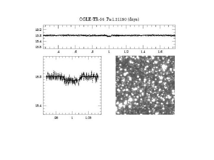
Search Strategies Strategy 2: Look at the galactic bulge with a large (1 -2 m) telescope (e. g. OGLE) Pros: Potentially many stars Cons: V-mag > 14 faint! Image in galactic bulge

Search Strategies Strategy 3: Look at a clusters with a large (1 -2 m) telescope Pros: Potentially many stars (depending on cluster) Cons: V-mag > 14 faint! Often not enough stars, most open clusters do not have 3000 -10000 stars Pleiades: open cluster M 92 globular cluster

Search Strategies Strategy 4: One star at a time! The MEarth project (http: //www. cfa. harvard. edu/~zberta/mearth/) uses 8 identical 40 cm telescopes to search for terrestrial planets around M dwarfs one after the other

Radial Velocity Follow-up for a Hot Jupiter The problem is not in finding the transits, the problem (bottleneck) is in confirming these with RVs which requires high resolution spectrographs. Telescope Easy Challenging Impossible 2 m V < 9 V=10 -12 V >13 4 m V < 10– 11 V=12 -14 V >15 8– 10 m V< 12– 14 V >17 V=14– 16 It takes approximately 8 -10 hours of telescope time on a large telescope to confirm one transit candidate

Summary 1. The Transit Method is an efficient way to find short period planets. 2. Combined with radial velocity measurements it gives you the mass, radius and thus density of planets 3. Roughly 1 in 3000 stars will have a transiting hot Jupiter → need to look at lots of stars (in galactic plane or clusters) 4. Radial Velocity measurements are essential to confirm planetary nature 5. a small telescope can do transit work (i. e even amateurs)