Transient Response First order system transient response Step

 + - 1 τs Y(s)")


 = 1 -y(t)=e-ptus(t) Normalized time t/t")


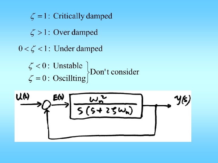


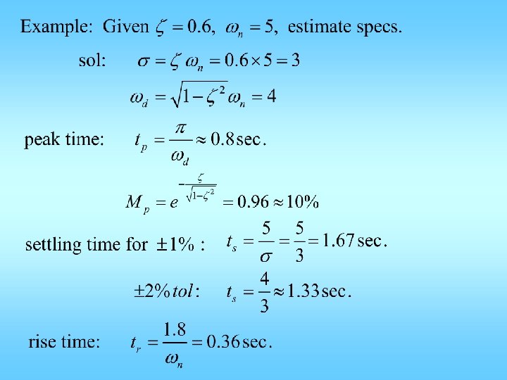
 Under damped, 0 < ζ < 1")
 q= tan-1(-Re/Im) s =-Re")
 max:")
)*100 plot(z, Mp) grid; Then")


/wn")
/wn Or about 2/wn")

 When ζ = 1, ωd = 0")

 Over damped: ζ > 1")


 area e. g. ζ >")


- Slides: 63
Transient Response • First order system transient response – Step response specs and relationship to pole location • Second order system transient response – Step response specs and relationship to pole location • Effects of additional poles and zeros
Prototype first order system E U(s) + - 1 τs Y(s)
First order system step resp Normalized time t/t
Prototype first order system • • • No overshoot, tp=inf, Mp = 0 Yss=1, ess=0 Settling time ts = [-ln(tol)]/p Delay time td = [-ln(0. 5)]/p Rise time tr = [ln(0. 9) – ln(0. 1)]/p • All times proportional to 1/p= t • Larger p means faster response
The error signal: e(t) = 1 -y(t)=e-ptus(t) Normalized time t/t
In every τ seconds, the error is reduced by 63. 2%
General First-order system We know how this responds to input Step response starts at y(0+)=k, final value kz/p 1/p = t is still time constant; in every t, y(t) moves 63. 2% closer to final value
Step response by MATLAB: >> p =. . >> n = [ b 1 b 0 ] >> d = [ 1 p ] >> step ( n , d ) Other MATLAB commands to explore: plot, hold, axis, xlabel, ylabel, title, text, gtext, semilogx, semilogy, loglog, subplot
Unit ramp response:
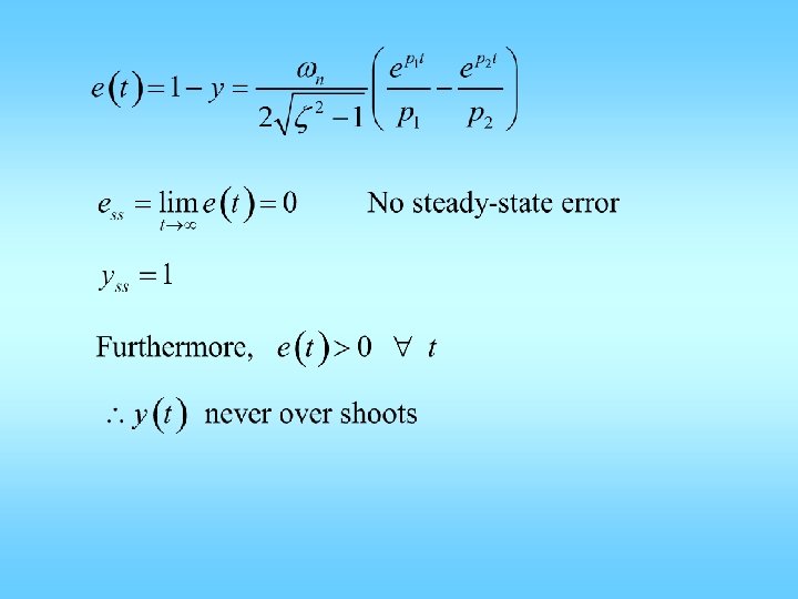
Note: In step response, the steady-state tracking error = zero.
Unit impulse response:
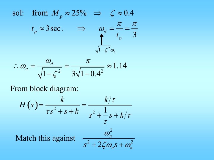
Prototype nd 2 order system:
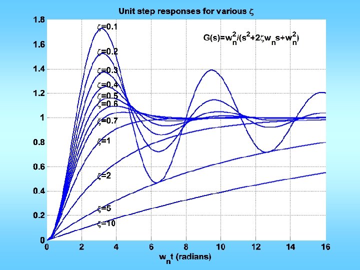
xi=[0. 7 1 2 5 10 0. 1 0. 2 0. 3 0. 4 0. 5 0. 6]; x=['zeta=0. 7'; 'zeta=1 '; 'zeta=2 '; 'zeta=5 '; 'zeta=10 '; 'zeta=0. 1'; 'zeta=0. 2'; 'zeta=0. 3'; 'zeta=0. 4'; 'zeta=0. 5'; 'zeta=0. 6']; T=0: 0. 01: 16; figure; hold; for k=1: length(xi) n=[1]; d=[1 2*xi(k) 1]; y=step(n, d, T); plot(T, y); if xi(k)>=0. 7 text(T(290), y(310), x(k, : )); else text(T(290), max(y)+0. 02, x(k, : )); end grid; end text(9, 1. 65, 'G(s)=w_n^2/(s^2+2zetaw_ns+w_n^2)') title('Unit step responses for various zeta') xlabel('w_nt (radians)') Can use omega in stead of w
annotation Create annotations including lines, arrows, text arrows, double arrows, text boxes, rectangles, and ellipses xlabel, ylabel, zlabel Add a text label to the respective axis title Add a title to a graph colorbar Add a colorbar to a graph legend Add a legend to a graph
For example: “help annotation” explains how to use the annotation command to add text, lines, arrows, and so on at desired positions in the graph ANNOTATION('textbox', POSITION) creates a textbox annotation at the position specified in normalized figure units by the vector POSITION ANNOTATION('line', X, Y) creates a line annotation with endpoints specified in normalized figure coordinates by the vectors X and Y ANNOTATION('arrow', X, Y) creates an arrow annotation with endpoints specified Example: ah=annotation('arrow', [. 9. 5], [. 9, . 5], 'Color', 'r'); th=annotation('textarrow', [. 3, . 6], [. 7, . 4], 'String', 'ABC');
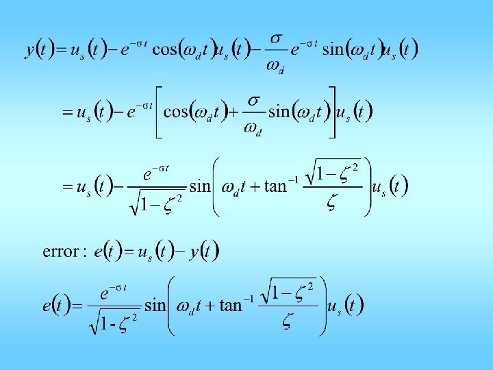
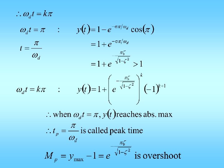
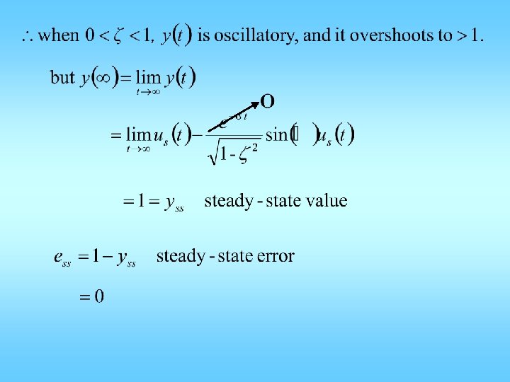
Unit step response: 1) Under damped, 0 < ζ < 1
d =Im cosq = z =-Re/|root| q= cos-1(Re/|root|) q= tan-1(-Re/Im) s =-Re
To find y(t) max:
z=0. 3: 0. 1: 0. 8; Mp=exp(-pi*z. /sqrt(1 -z. *z))*100 plot(z, Mp) grid; Then preference -> figure… ->powerpoint -> apply to figure Then copy figure
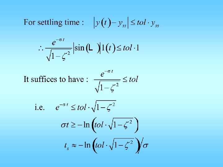
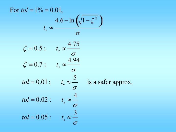
For 5% tolerance Ts ~= 3/zwn
• Delay time is not used very much • For delay time, solve y(t)=0. 5 and solve for t • For rise time, set y(t) = 0. 1 & 0. 9, solve for t • This is very difficult • Based on numerical simulation:
Useful Range Td=(0. 8+0. 9 z)/wn
Useful Range Tr=4. 5(z-0. 2)/wn Or about 2/wn
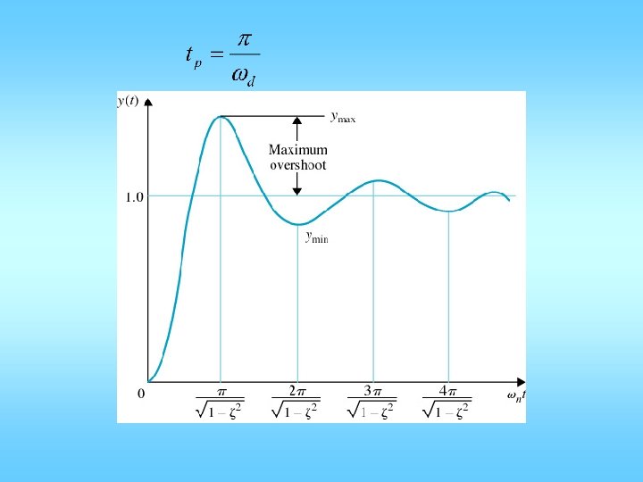
Putting all things together: Settling time:
2) When ζ = 1, ωd = 0
The tracking error:
3) Over damped: ζ > 1
Transient Response Recall 1 st order system step response: 2 nd order:
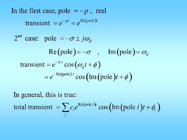
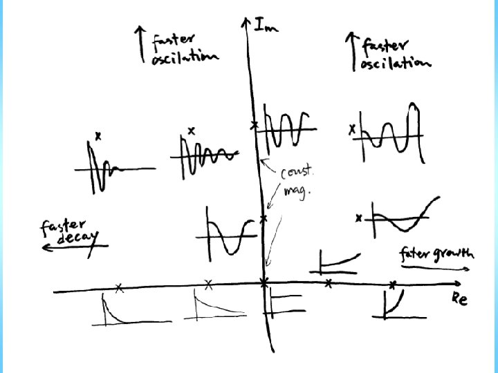
Pole location determines transient
• All closed-loop poles must be strictly in the left half planes Transient dies away • Dominant poles: the single real pole or the complex pole pair which contribute the most to the transient • Typically have dominant pole pair – (complex conjugate) – Closest to jω-axis (i. e. the least negative) – Slowest to die away
Typical design specifications • Steady-state: ess to step ≤ # % ts ≤ · · · • Speed (responsiveness) tr ≤ · · · td ≤ · · · • Relative stability Mp ≤ · · · %
These specs translate into requirements on ζ, ωn or on closed-loop pole location : Find ranges for ζ and ωn so that all 3 are satisfied.
Find conditions on σ and ωd.
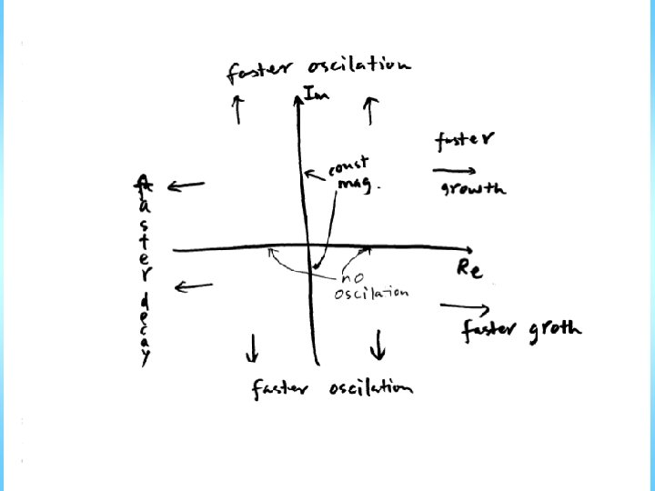
In the complex plane :
Constant σ : vertical lines σ > # is half plane
Constant ωd : horizontal line ωd < · · · is a band ωd > · · · is the plane excluding band
Constant ωn : circles ωn < · · · inside of a circle ωn > · · · outside of a circle
Constant ζ : φ = cos-1ζ constant Constant ζ = ray from the origin ζ > · · · is the cone ζ < · · · is the other part
If more than one requirement, get the common (overlapped) area e. g. ζ > 0. 5, σ > 2, ωn > 3 gives Sometimes meeting two will also meet the third, but not always.
Try to remember these:
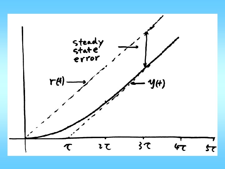
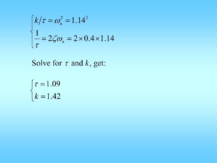
Example: + - When given unit step input, the output looks like: Q: estimate k and τ.
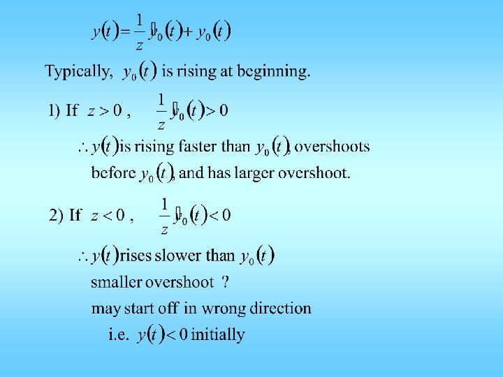
Effects of additional zeros Suppose we originally have: i. e. step response Now introduce a zero at s = -z The new step response:
Effects: • Increased speed, • Larger overshoot, • Might increase ts
When z < 0, the zero s = -z is > 0, is in the right half plane. Such a zero is called a nonminimum phase zero. A system with nonminimum phase zeros is called a nonminimum phase system. Nonminimum phase zero should be avoided in design. i. e. Do not introduce such a zero in your controller.
Effects of additional pole Suppose, instead of a zero, we introduce a pole at s = -p, i. e.
L. P. F. has smoothing effect, or averaging effect Effects: • Slower, • Reduced overshoot, • May increase or decrease ts