Transient Response and SteadyState Response The time response

Transient Response and Steady-State Response. The time response of a control system consists of two parts: - the transient response - and the steady-state response. By transient response, we mean that which goes from the initial state to the final state. By steady-state response, we mean the manner in which the system output behaves as t approaches infinity. Thus the system response c(t) may be written as c(t) = ctr(t) + css(t)

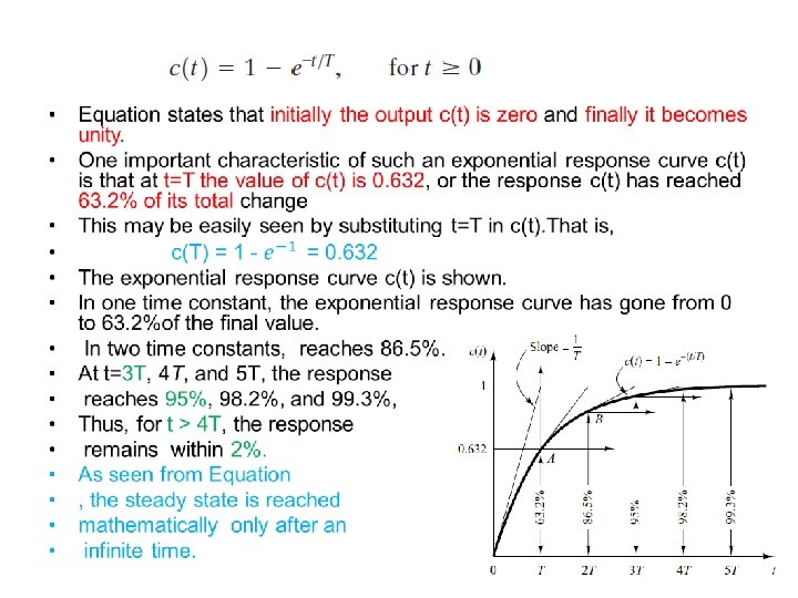
FIRST-ORDER SYSTEMS • Consider the first-order system shown in Figure 5– 1(a). Physically, this system may represent an RC circuit, thermal system, or the like • Unit-Step Response of First-Order Systems. Since the Laplace transform of the unit-step function is 1/s, substituting R(s)=1/s into Equation, we obtain

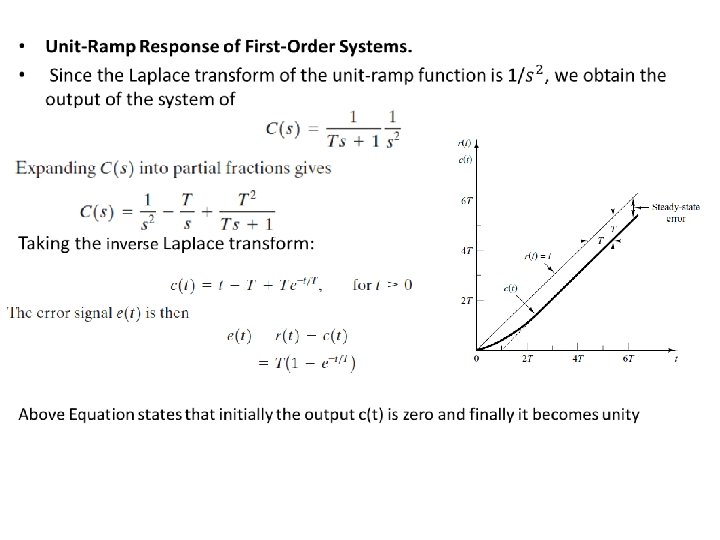
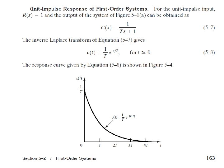
• for the unit-ramp input the output c(t) is • For the unit-step input, which is the derivative of unit-ramp input, the output c(t) is • Finally, for the unit-impulse input, which is the derivative of unit-step input, the output c(t) is

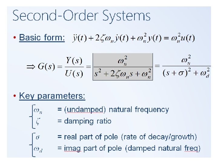
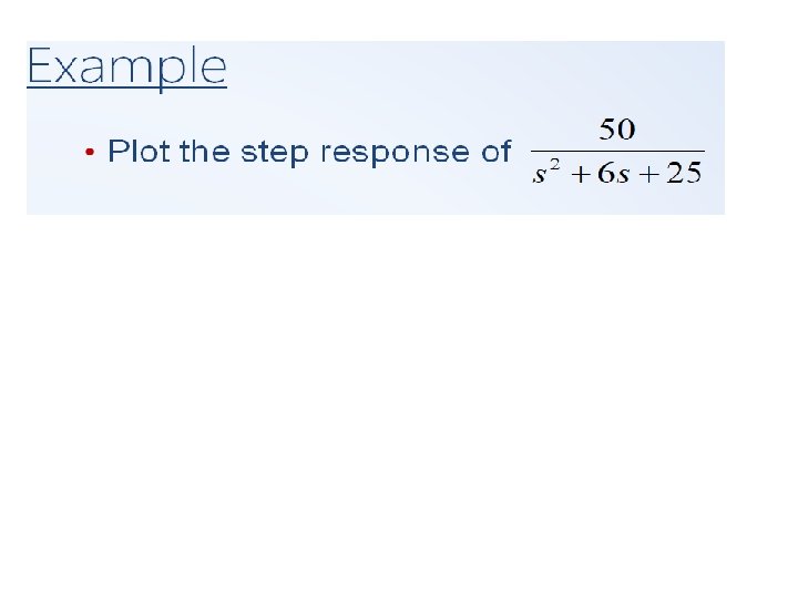
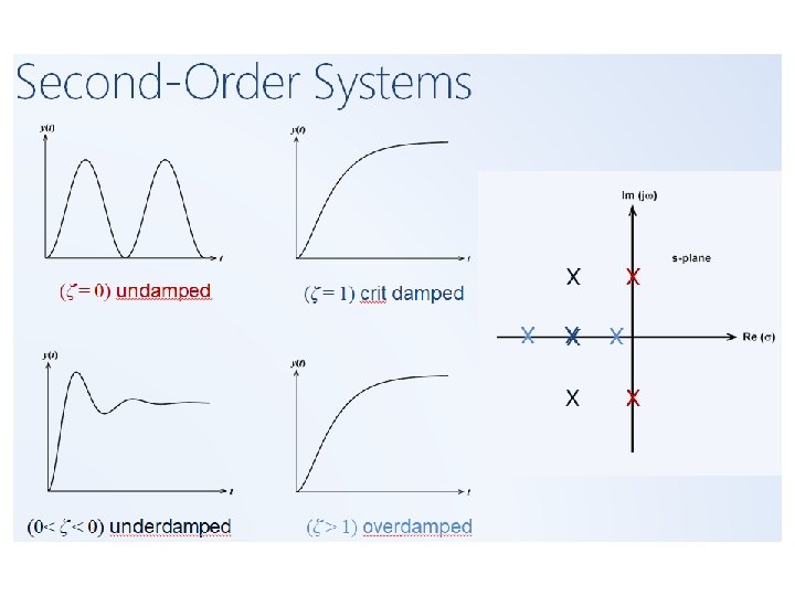
Second-Order Systems

• First-Order Systems: • Step Response:

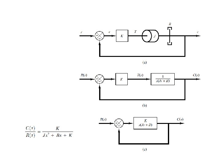
Second-Order Systems • Servo System. The servo system shown in Figure consists of a proportional • controller and load elements (inertia and viscous-friction elements). Suppose that we wish to control the output position c in accordance with the input position r. The equation for the load elements is

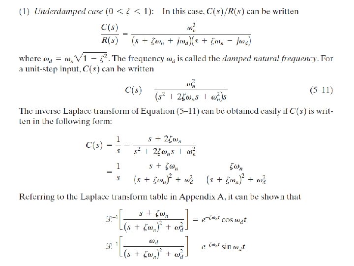
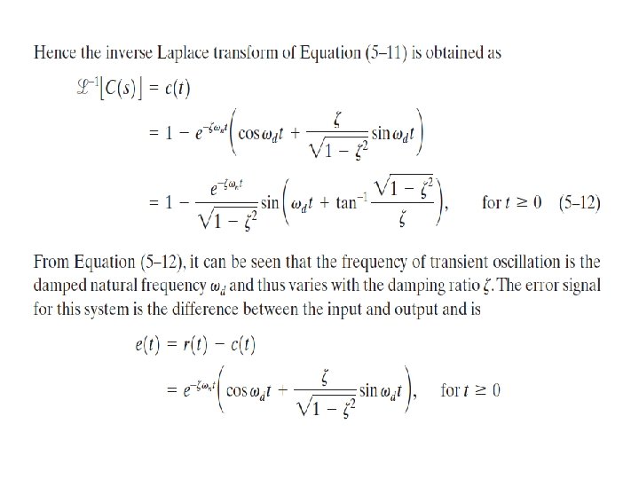
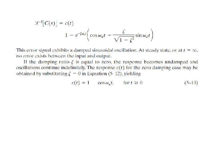
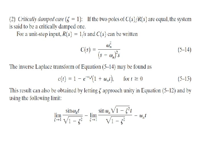
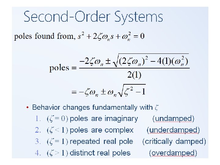
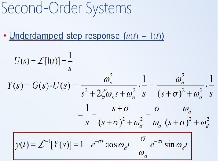
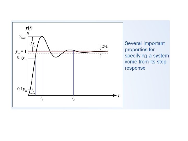
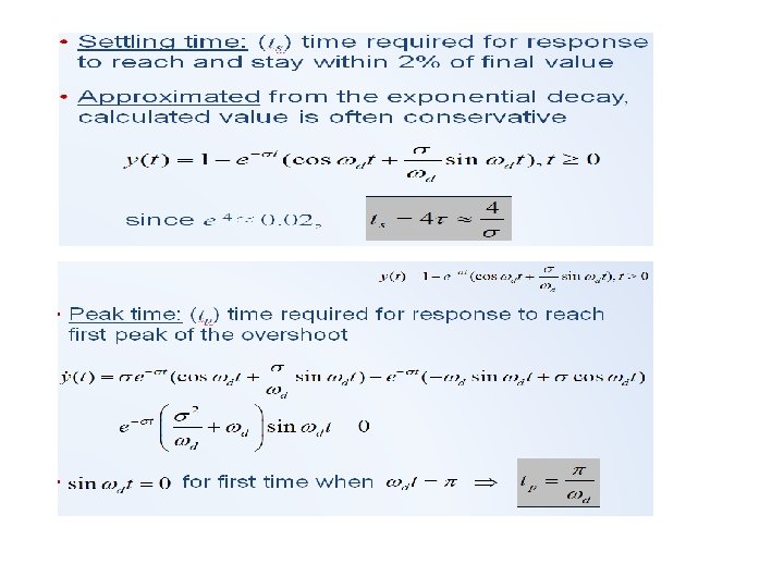
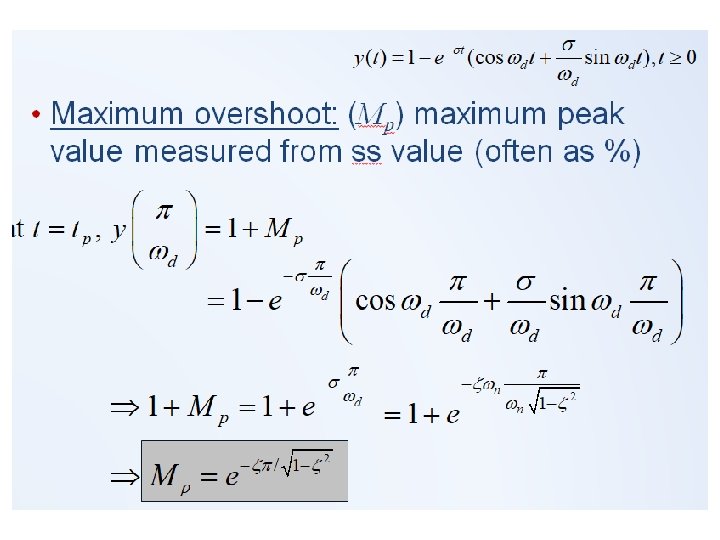
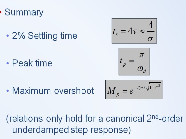
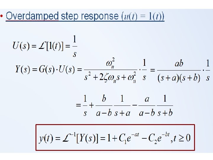
• Step Response of Second-Order System. • The closed-loop transfer function of • the system shown • Which can be written as: • ; ; • This form is called the standard form of the second-order system • The dynamic behavior of the second-order • system can then be described in terms of • two parameters and ωn. ;

When z is appreciably greater than unity, one of the two decaying exponentials decreases much faster than the other, so the faster-decaying exponential term (which corresponds to a smaller time constant) may be neglected. That is, if –s 2 is located very much closer to the jω axis than –s 1. which means s 2 <<s 1 , then for an approximate solution we may neglect –s 1

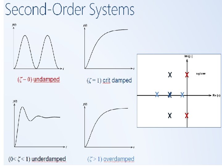
• Pole locations determine time response

• EXAMPLE 5– 2 For the system shown in Figure , determine the values of gain K and velocity-feedback constant Kh so that the maximum overshoot in the unit-step response is 0. 2 and the peak time is 1 sec. With these values of K and Kh, obtain the rise time and settling time. Assume that J=1 kg-m 2 and B=1 N-m/ rad/ sec. • Example: When the system shown in Figure (a) is subjected to a unit-step input, the system output responds as shown in Figure (b). Determine the values of K and T from the response curve.

• Example: Determine the values of K and k of the closed-loop system shown in Figure so that the maximum overshoot in unit-step response is 25% and the peak time is 2 sec. Assume that J=1 kg-m 2.