Transforms Hierarchical Modeling Scene Graphs Using hierarchical modeling

Transforms Hierarchical Modeling Scene Graphs Using hierarchical modeling techniques in 3 D software design l. Transforms l. Local basis l Matrix math review l Matrices and Open. GL l Hierarchical modeling l Benefits of hierarchical modeling l Hierarchical modeling in C++ and Open. GL l Recursive Hierarchical modeling

What does it mean to talk about the center of the world? “Giant Turtle”, from the Discworld series. Image (c) Jay Hurst

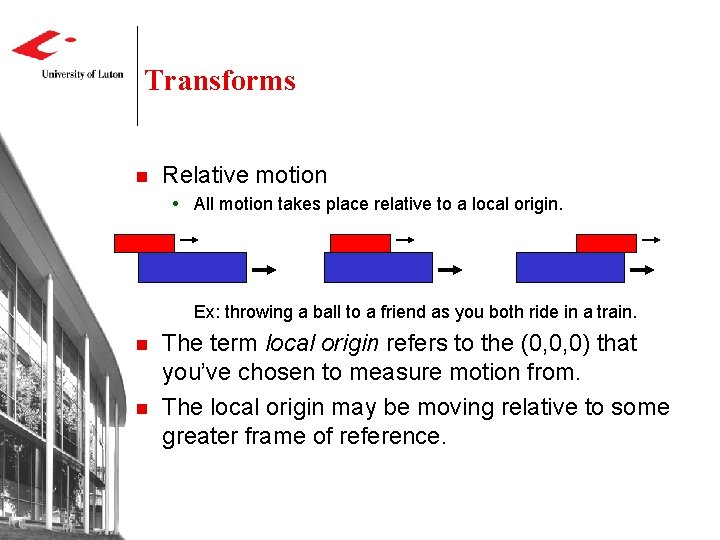
Transforms n Relative motion All motion takes place relative to a local origin. Ex: throwing a ball to a friend as you both ride in a train. n n The term local origin refers to the (0, 0, 0) that you’ve chosen to measure motion from. The local origin may be moving relative to some greater frame of reference.

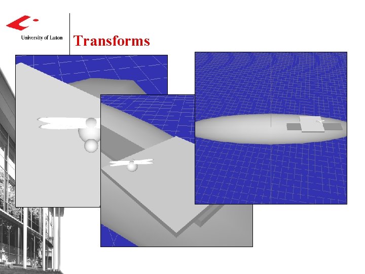
Transforms

Transforms n The following terms are used more-or-less interchangeably: Local basis Local transform Frame of reference n Each of these refers to the location, in the greater world, of the (0, 0, 0) you’re working with. They also include the concept of the current basis, which is the X, Y, Z directions. By rotating the basis of a coordinate system, you can rotate the world it describes.

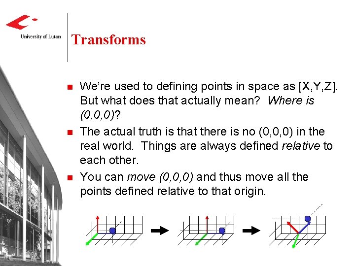
Transforms n n n We’re used to defining points in space as [X, Y, Z]. But what does that actually mean? Where is (0, 0, 0)? The actual truth is that there is no (0, 0, 0) in the real world. Things are always defined relative to each other. You can move (0, 0, 0) and thus move all the points defined relative to that origin.

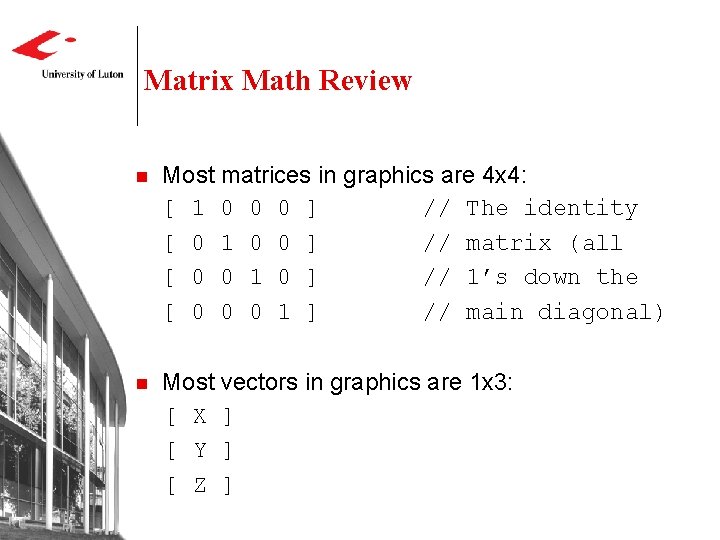
Matrix Math Review n Most matrices in graphics are 4 x 4: [ 1 0 0 0 ] // The identity [ 0 1 0 0 ] // matrix (all [ 0 0 1 0 ] // 1’s down the [ 0 0 0 1 ] // main diagonal) n Most vectors in graphics are 1 x 3: [ X ] [ Y ] [ Z ]

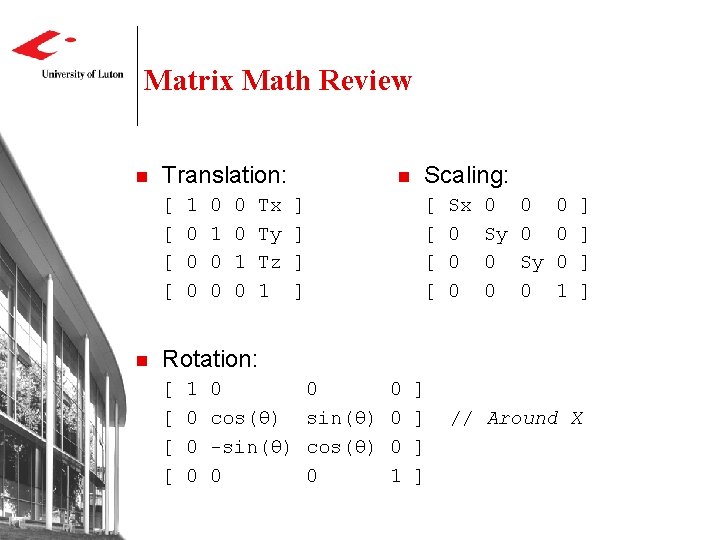
Matrix Math Review n Translation: [ [ n 1 0 0 0 0 1 0 Tx Ty Tz 1 n ] ] Scaling: [ [ Sx 0 0 0 0 Sy 0 0 1 ] ] Rotation: [ [ 1 0 0 cos(θ) -sin(θ) 0 0 sin(θ) cos(θ) 0 0 1 ] ] // Around X

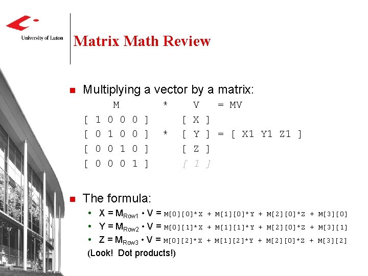
Matrix Math Review n Multiplying a vector by a matrix: M [ [ n 1 0 0 * 0 0 1 ] ] * [ [ V X Y Z 1 = MV ] ] = [ X 1 Y 1 Z 1 ] ] ] The formula: X = MRow 1 • V = M[0][0]*X Y = MRow 2 • V = M[0][1]*X Z = MRow 3 • V = M[0][2]*X (Look! Dot products!) + M[1][0]*Y + M[2][0]*Z + M[3][0] + M[1][1]*Y + M[2][0]*Z + M[3][1] + M[1][2]*Y + M[2][0]*Z + M[3][2]

Matrix Math Review n Multiplying a matrix by a matrix: [ [ n 1 0 0 0 0 1 ] [ 1 ] * [ 0 ] [ 0 The formula: M M[col a][row b] 0 1 0 0 0 0 1 ] [ 1 ] = [ 0 ] [ 0 0 1 0 0 0 0 1 ] ] = M 1 * M 2 = M 1(row a) • M 2(col b)

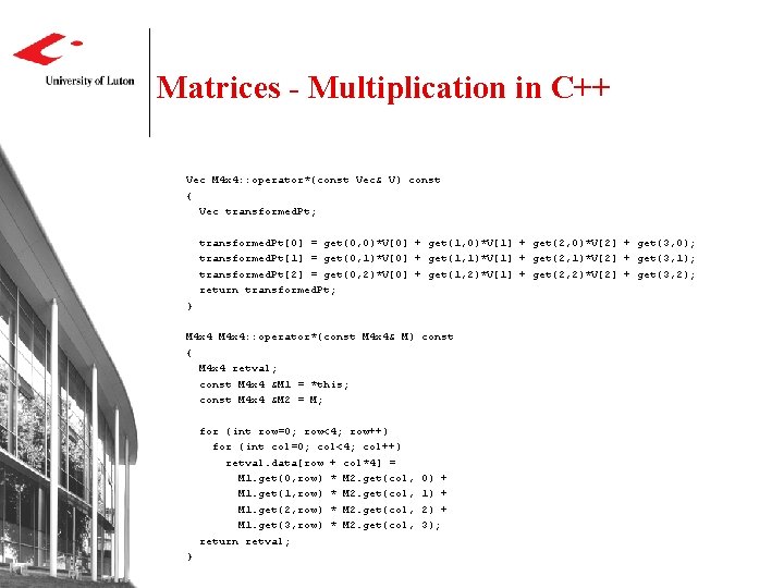
Matrices - Multiplication in C++ Vec M 4 x 4: : operator*(const Vec& V) const { Vec transformed. Pt; transformed. Pt[0] = get(0, 0)*V[0] + get(1, 0)*V[1] + get(2, 0)*V[2] + get(3, 0); transformed. Pt[1] = get(0, 1)*V[0] + get(1, 1)*V[1] + get(2, 1)*V[2] + get(3, 1); transformed. Pt[2] = get(0, 2)*V[0] + get(1, 2)*V[1] + get(2, 2)*V[2] + get(3, 2); return transformed. Pt; } M 4 x 4: : operator*(const M 4 x 4& M) const { M 4 x 4 retval; const M 4 x 4 &M 1 = *this; const M 4 x 4 &M 2 = M; for (int row=0; row<4; row++) for (int col=0; col<4; col++) retval. data[row + col*4] = M 1. get(0, row) * M 2. get(col, M 1. get(1, row) * M 2. get(col, M 1. get(2, row) * M 2. get(col, M 1. get(3, row) * M 2. get(col, return retval; } 0) + 1) + 2) + 3);

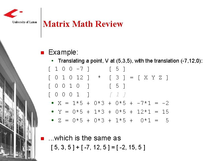
Matrix Math Review n Example: Translating a point, V at (5, 3, 5), with the translation (-7, 12, 0): [ [ 1 0 0 -7 0 12 0 0 1 X = 1*5 Y = 0*5 Z = 0*5 n ] [ 5 ] ] * [ 3 ] ] [ 5 ] ] [ 1 ] + 0*3 + 0*5 + 1*3 + 0*5 + 0*3 + 1*5 = [ X Y Z ] + -7*1 = -2 + 12*1 = 15 + 0*1 = 5 . . . which is the same as [ 5, 3, 5 ] + [ -7, 12, 5 ] = [ -2, 15, 5 ]

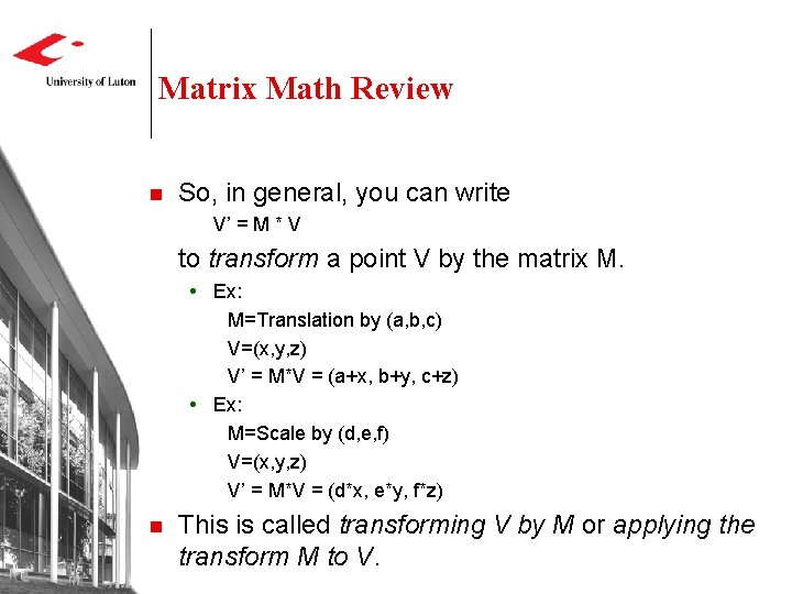
Matrix Math Review n So, in general, you can write V’ = M * V to transform a point V by the matrix M. Ex: M=Translation by (a, b, c) V=(x, y, z) V’ = M*V = (a+x, b+y, c+z) Ex: M=Scale by (d, e, f) V=(x, y, z) V’ = M*V = (d*x, e*y, f*z) n This is called transforming V by M or applying the transform M to V.

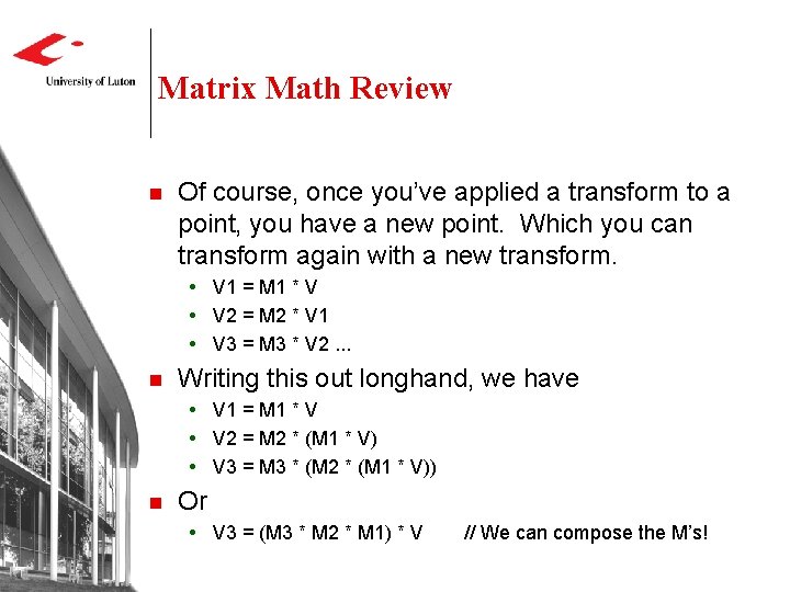
Matrix Math Review n Of course, once you’ve applied a transform to a point, you have a new point. Which you can transform again with a new transform. V 1 = M 1 * V V 2 = M 2 * V 1 V 3 = M 3 * V 2. . . n Writing this out longhand, we have V 1 = M 1 * V V 2 = M 2 * (M 1 * V) V 3 = M 3 * (M 2 * (M 1 * V)) n Or V 3 = (M 3 * M 2 * M 1) * V // We can compose the M’s!

Matrix Math Review n This key idea--that you can compose multiple transforms before applying them to a point-makes it possible to do all sorts of wonderful optimizations. You can build up a series of transformations and compose them together into a single matrix which rotates and translates and rotates again, then scales and translates once more. The order of operations is preserved in the composed matrix. The order of the original operations is preserved in the composed matrix exactly as originally entered. This means that you can build a single matrix which contains within its values an arbitrary sequence of translations, rotations and scales. And you can apply that matrix to your 3 D models, to move them about.

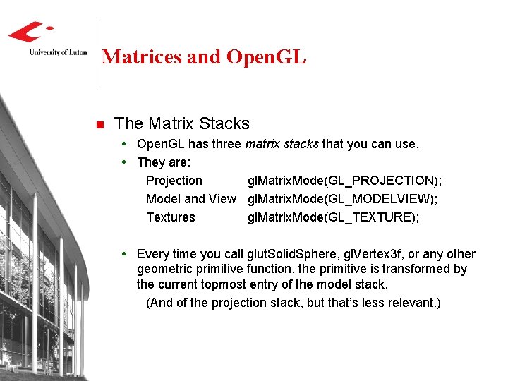
Matrices and Open. GL n The Matrix Stacks Open. GL has three matrix stacks that you can use. They are: Projection gl. Matrix. Mode(GL_PROJECTION); Model and View gl. Matrix. Mode(GL_MODELVIEW); Textures gl. Matrix. Mode(GL_TEXTURE); Every time you call glut. Solid. Sphere, gl. Vertex 3 f, or any other geometric primitive function, the primitive is transformed by the current topmost entry of the model stack. (And of the projection stack, but that’s less relevant. )

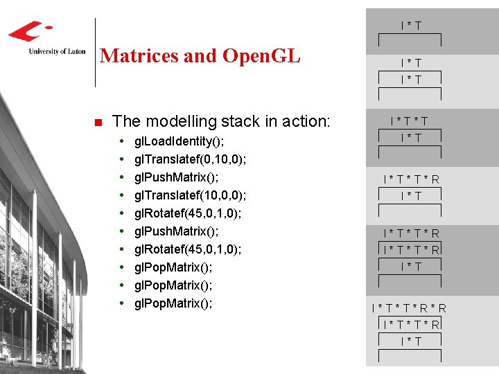
I*T Matrices and Open. GL n The modelling stack in action: gl. Load. Identity(); gl. Translatef(0, 10, 0); gl. Push. Matrix(); gl. Translatef(10, 0, 0); gl. Rotatef(45, 0, 1, 0); gl. Push. Matrix(); gl. Rotatef(45, 0, 1, 0); gl. Pop. Matrix(); I*T I*T*T*R I*T*T*R I*T I*T*T*R*R I*T*T*R I*T

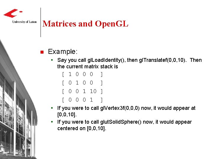
Matrices and Open. GL n Example: Say you call gl. Load. Identity(), then gl. Translatef(0, 0, 10). Then the current matrix stack is [ [ 1 0 0 0 0 10 1 ] ] If you were to call gl. Vertex 3 f(0, 0, 0) now, it would appear at [0, 0, 10]. If you were to call glut. Solid. Sphere() now, it would appear centered on [0, 0, 10].

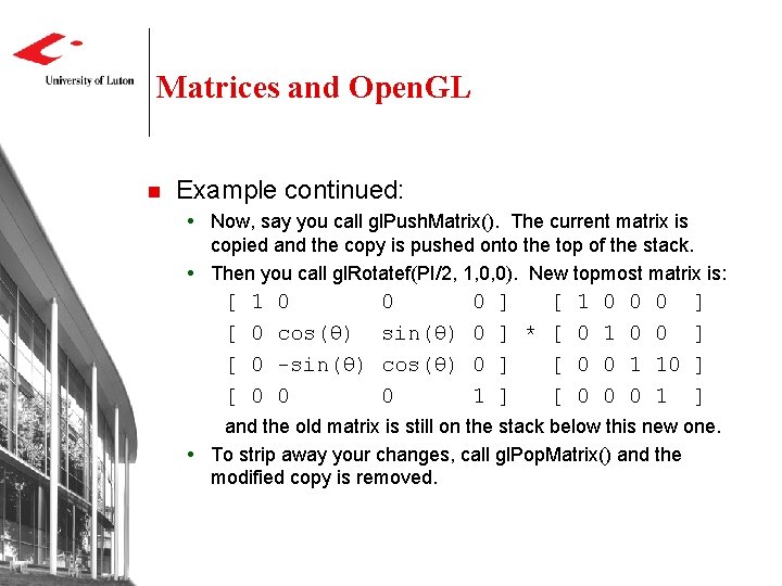
Matrices and Open. GL n Example continued: Now, say you call gl. Push. Matrix(). The current matrix is copied and the copy is pushed onto the top of the stack. Then you call gl. Rotatef(PI/2, 1, 0, 0). New topmost matrix is: [ [ 1 0 0 cos(θ) -sin(θ) 0 0 sin(θ) cos(θ) 0 0 1 ] [ 1 ] * [ 0 ] [ 0 0 1 0 0 0 10 1 ] ] and the old matrix is still on the stack below this new one. To strip away your changes, call gl. Pop. Matrix() and the modified copy is removed.

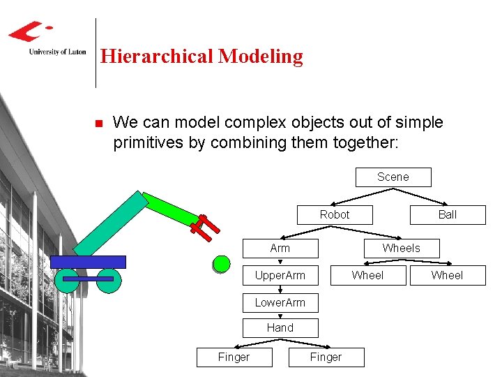
Hierarchical Modeling n We can model complex objects out of simple primitives by combining them together: Scene Robot Arm Wheels Upper. Arm Wheel Lower. Arm Hand Finger Ball Finger Wheel

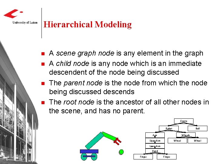
Hierarchical Modeling n n A scene graph node is any element in the graph A child node is any node which is an immediate descendent of the node being discussed The parent node is the node from which the node being discussed descends The root node is the ancestor of all other nodes in the scene, and has no parent. Scene Robot Ball Arm Wheels Upper. Arm Wheel Lower. Arm Hand Finger Wheel

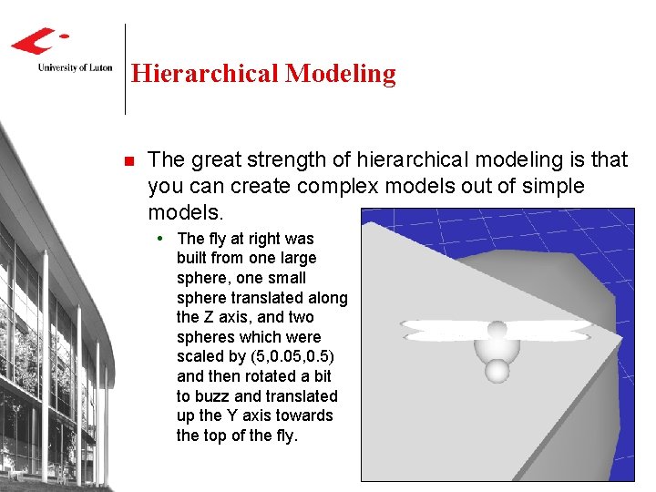
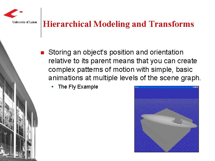
Hierarchical Modeling n The great strength of hierarchical modeling is that you can create complex models out of simple models. The fly at right was built from one large sphere, one small sphere translated along the Z axis, and two spheres which were scaled by (5, 0. 05, 0. 5) and then rotated a bit to buzz and translated up the Y axis towards the top of the fly.

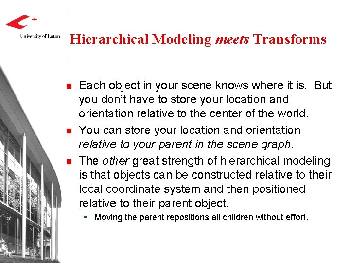
Hierarchical Modeling meets Transforms n n n Each object in your scene knows where it is. But you don’t have to store your location and orientation relative to the center of the world. You can store your location and orientation relative to your parent in the scene graph. The other great strength of hierarchical modeling is that objects can be constructed relative to their local coordinate system and then positioned relative to their parent object. Moving the parent repositions all children without effort.

Hierarchical Modeling and Transforms n Storing an object’s position and orientation relative to its parent means that you can create complex patterns of motion with simple, basic animations at multiple levels of the scene graph. The Fly Example

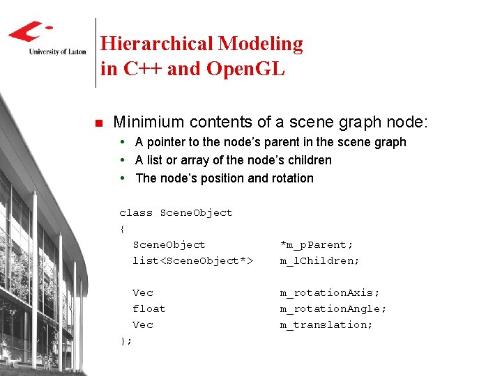
Hierarchical Modeling in C++ and Open. GL n Minimium contents of a scene graph node: A pointer to the node’s parent in the scene graph A list or array of the node’s children The node’s position and rotation class Scene. Object { Scene. Object list<Scene. Object*> Vec float Vec }; *m_p. Parent; m_l. Children; m_rotation. Axis; m_rotation. Angle; m_translation;

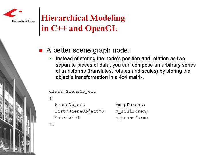
Hierarchical Modeling in C++ and Open. GL n A better scene graph node: Instead of storing the node’s position and rotation as two separate pieces of data, you can compose an arbitrary series of transforms (translates, rotates and scales) by storing the object’s transformation in a 4 x 4 matrix. class Scene. Object { Scene. Object list<Scene. Object*> Matrix 4 x 4 }; *m_p. Parent; m_l. Children; m_transform;

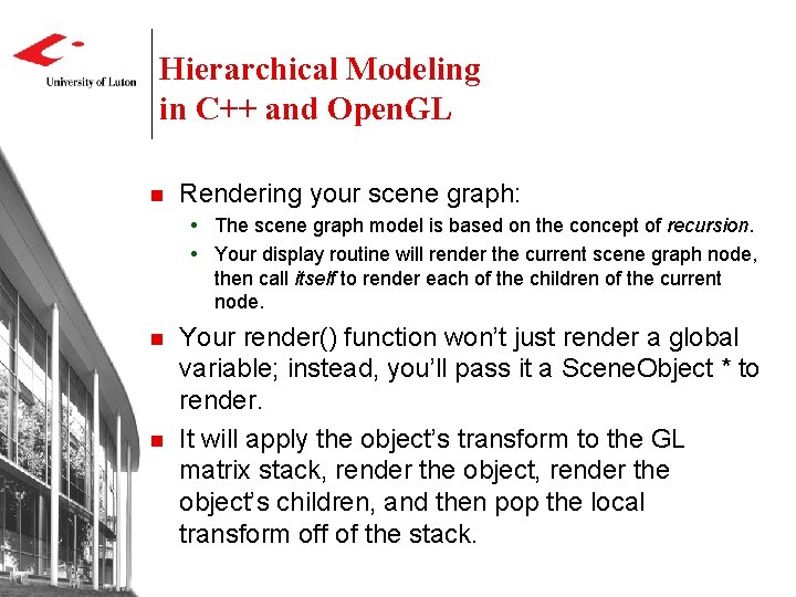
Hierarchical Modeling in C++ and Open. GL n Rendering your scene graph: The scene graph model is based on the concept of recursion. Your display routine will render the current scene graph node, then call itself to render each of the children of the current node. n n Your render() function won’t just render a global variable; instead, you’ll pass it a Scene. Object * to render. It will apply the object’s transform to the GL matrix stack, render the object’s children, and then pop the local transform off of the stack.

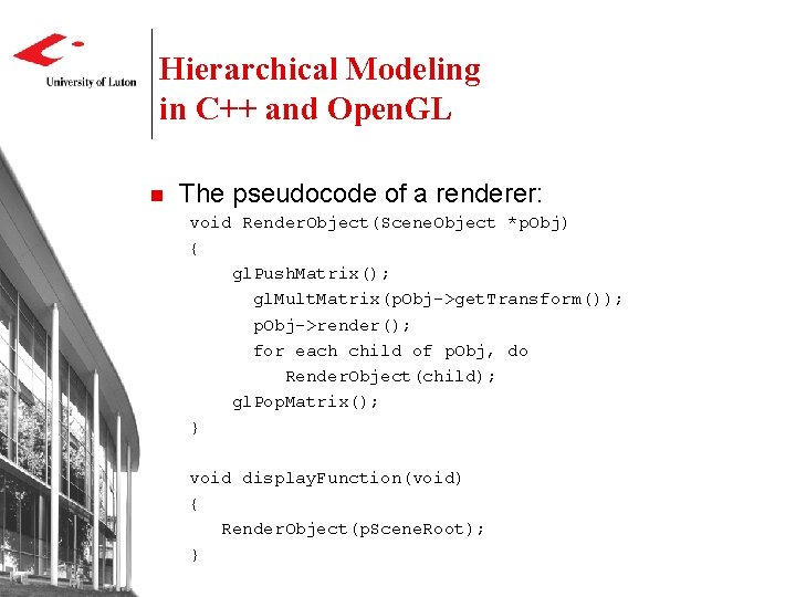
Hierarchical Modeling in C++ and Open. GL n The pseudocode of a renderer: void Render. Object(Scene. Object *p. Obj) { gl. Push. Matrix(); gl. Mult. Matrix(p. Obj->get. Transform()); p. Obj->render(); for each child of p. Obj, do Render. Object(child); gl. Pop. Matrix(); } void display. Function(void) { Render. Object(p. Scene. Root); }

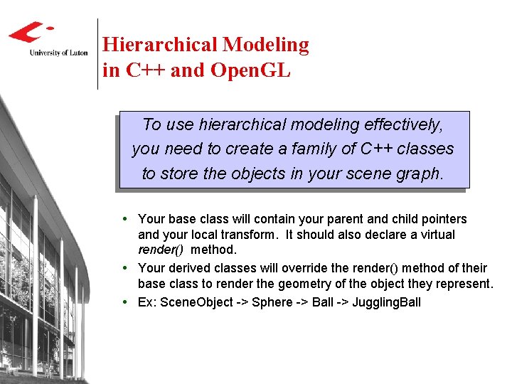
Hierarchical Modeling in C++ and Open. GL To use hierarchical modeling effectively, you need to create a family of C++ classes to store the objects in your scene graph. Your base class will contain your parent and child pointers and your local transform. It should also declare a virtual render() method. Your derived classes will override the render() method of their base class to render the geometry of the object they represent. Ex: Scene. Object -> Sphere -> Ball -> Juggling. Ball

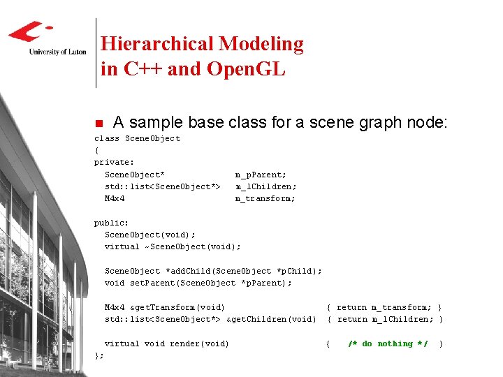
Hierarchical Modeling in C++ and Open. GL n A sample base class for a scene graph node: class Scene. Object { private: Scene. Object* std: : list<Scene. Object*> M 4 x 4 m_p. Parent; m_l. Children; m_transform; public: Scene. Object(void); virtual ~Scene. Object(void); Scene. Object *add. Child(Scene. Object *p. Child); void set. Parent(Scene. Object *p. Parent); }; M 4 x 4 &get. Transform(void) std: : list<Scene. Object*> &get. Children(void) { return m_transform; } { return m_l. Children; } virtual void render(void) { /* do nothing */ }

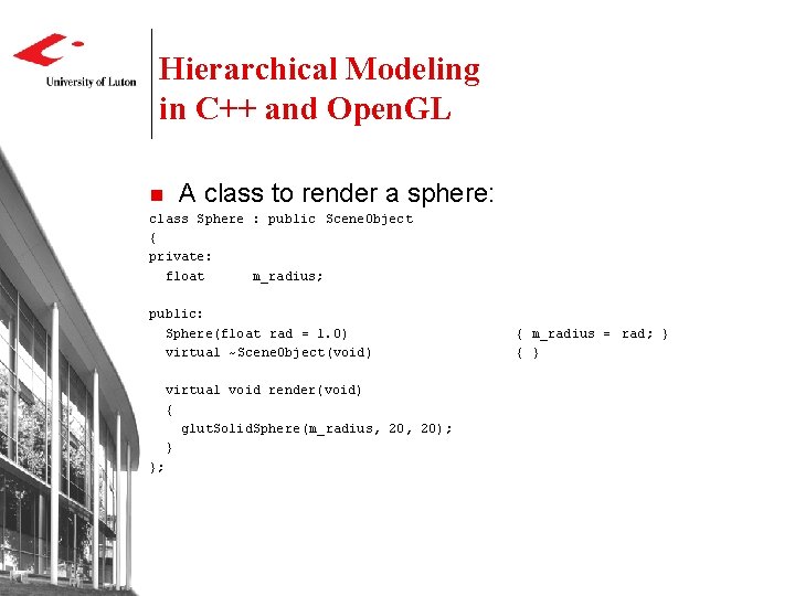
Hierarchical Modeling in C++ and Open. GL n A class to render a sphere: class Sphere : public Scene. Object { private: float m_radius; public: Sphere(float rad = 1. 0) virtual ~Scene. Object(void) virtual void render(void) { glut. Solid. Sphere(m_radius, 20); } }; { m_radius = rad; } { }

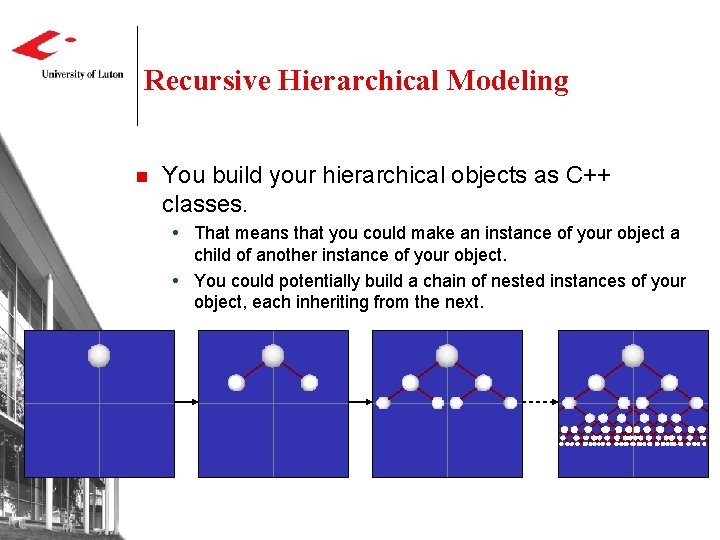
Recursive Hierarchical Modeling n You build your hierarchical objects as C++ classes. That means that you could make an instance of your object a child of another instance of your object. You could potentially build a chain of nested instances of your object, each inheriting from the next.

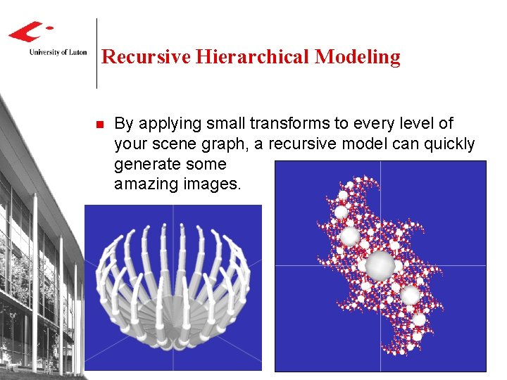
Recursive Hierarchical Modeling n By applying small transforms to every level of your scene graph, a recursive model can quickly generate some amazing images.