Transformations With Open GL Courtesy of Drs Carol

Transformations With Open. GL Courtesy of Drs. Carol O’Sullivan / Yann Morvan Trinity College Dublin

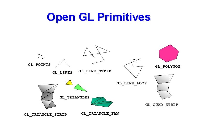
Open GL Primitives

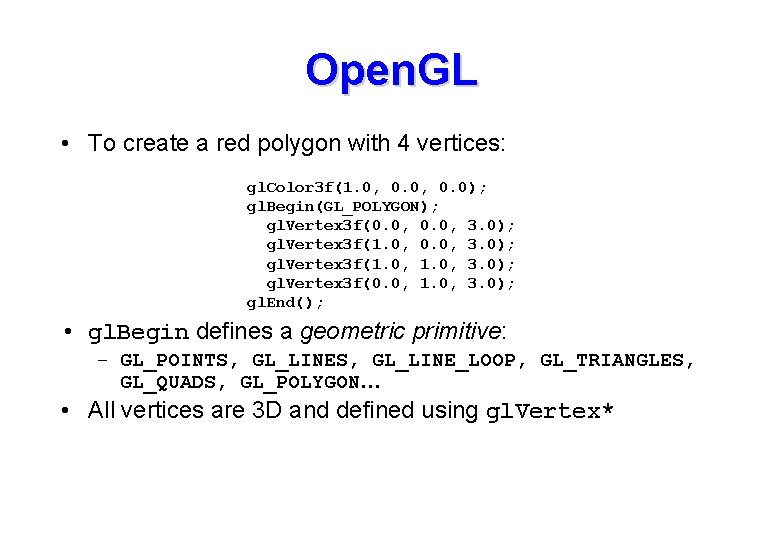
Open. GL • To create a red polygon with 4 vertices: gl. Color 3 f(1. 0, 0. 0); gl. Begin(GL_POLYGON); gl. Vertex 3 f(0. 0, 3. 0); gl. Vertex 3 f(1. 0, 3. 0); gl. Vertex 3 f(0. 0, 1. 0, 3. 0); gl. End(); • gl. Begin defines a geometric primitive: – GL_POINTS, GL_LINE_LOOP, GL_TRIANGLES, GL_QUADS, GL_POLYGON… • All vertices are 3 D and defined using gl. Vertex*

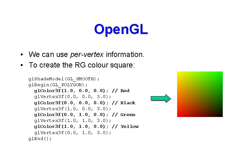
Open. GL • We can use per-vertex information. • To create the RG colour square: gl. Shade. Model(GL_SMOOTH); gl. Begin(GL_POLYGON); gl. Color 3 f(1. 0, 0. 0); // gl. Vertex 3 f(0. 0, 3. 0); gl. Color 3 f(0. 0, 0. 0); // gl. Vertex 3 f(1. 0, 0. 0, 3. 0); gl. Color 3 f(0. 0, 1. 0, 0. 0); // gl. Vertex 3 f(1. 0, 3. 0); gl. Color 3 f(1. 0, 0. 0); // gl. Vertex 3 f(0. 0, 1. 0, 3. 0); gl. End(); Red Black Green Yellow

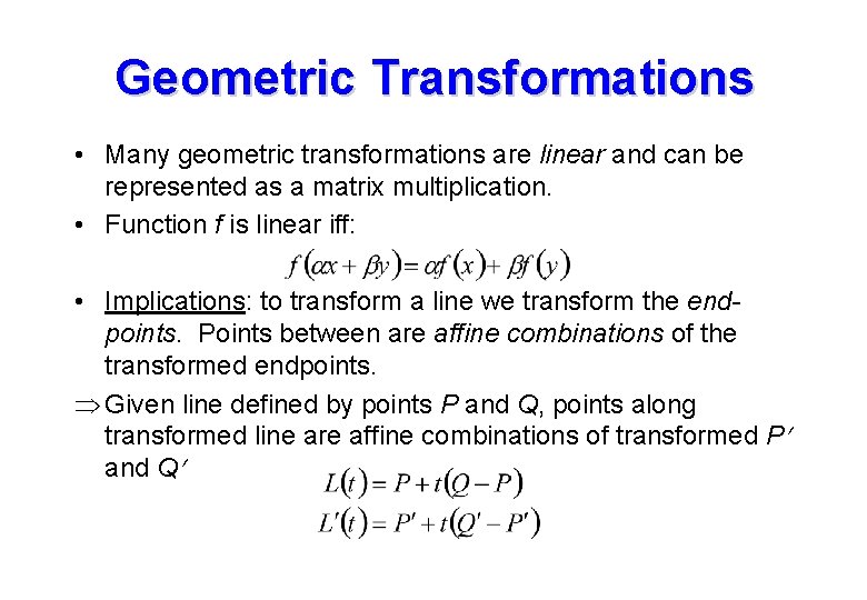
Geometric Transformations • Many geometric transformations are linear and can be represented as a matrix multiplication. • Function f is linear iff: • Implications: to transform a line we transform the endpoints. Points between are affine combinations of the transformed endpoints. Given line defined by points P and Q, points along transformed line are affine combinations of transformed P and Q

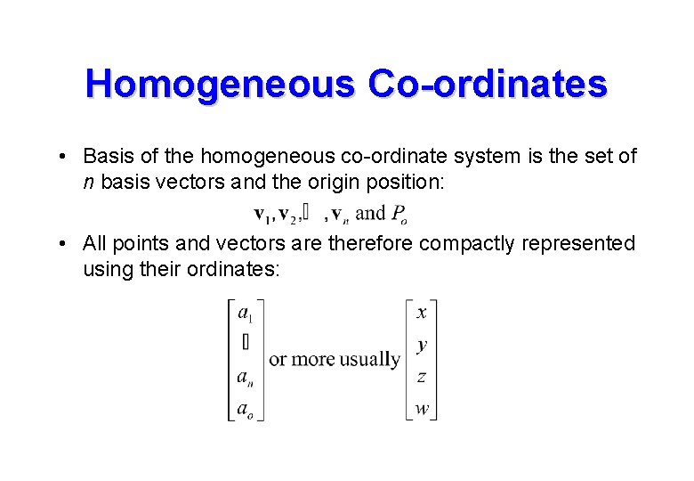
Homogeneous Co-ordinates • Basis of the homogeneous co-ordinate system is the set of n basis vectors and the origin position: • All points and vectors are therefore compactly represented using their ordinates:

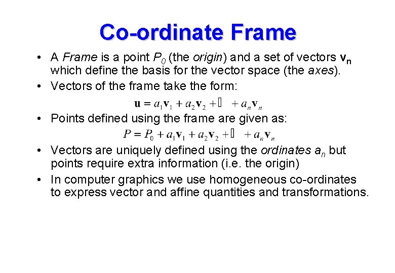
Co-ordinate Frame • A Frame is a point P 0 (the origin) and a set of vectors vn which define the basis for the vector space (the axes). • Vectors of the frame take the form: • Points defined using the frame are given as: • Vectors are uniquely defined using the ordinates an but points require extra information (i. e. the origin) • In computer graphics we use homogeneous co-ordinates to express vector and affine quantities and transformations.

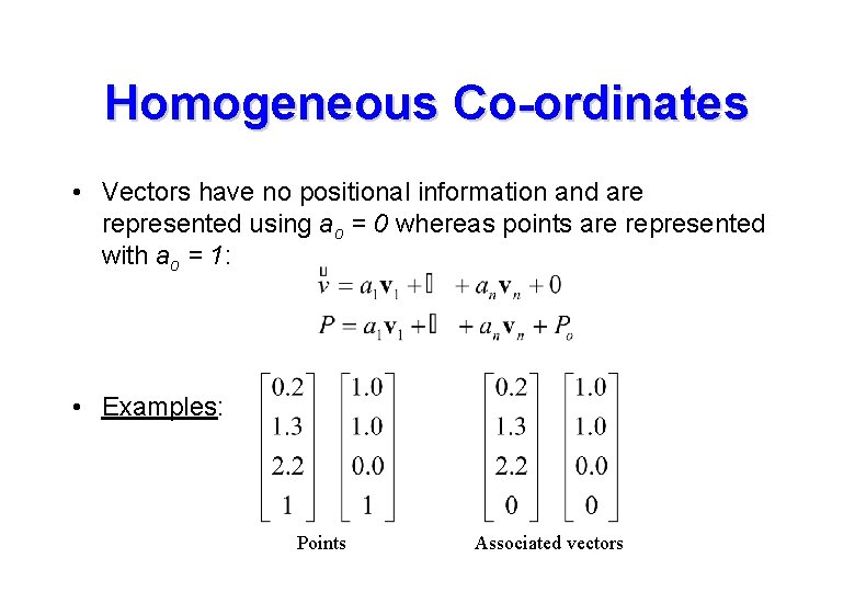
Homogeneous Co-ordinates • Vectors have no positional information and are represented using ao = 0 whereas points are represented with ao = 1: • Examples: Points Associated vectors

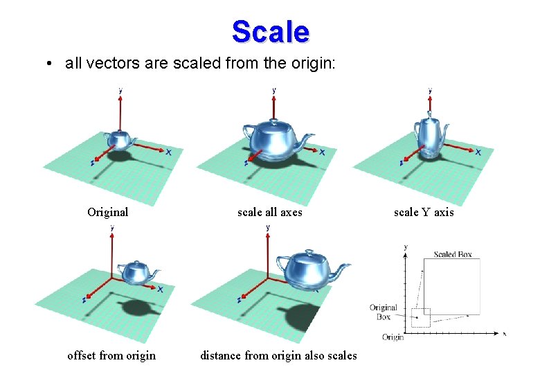
Scale • all vectors are scaled from the origin: Original offset from origin scale all axes distance from origin also scales scale Y axis

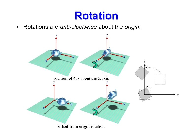
Rotation • Rotations are anti-clockwise about the origin: rotation of 45 o about the Z axis offset from origin rotation

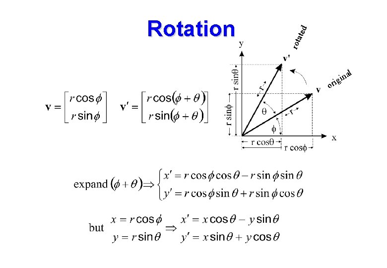
ted rota Rotation or al n i ig

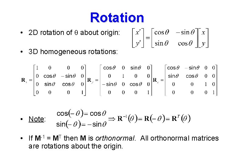
Rotation • 2 D rotation of q about origin: • 3 D homogeneous rotations: • Note: • If M-1 = MT then M is orthonormal. All orthonormal matrices are rotations about the origin.

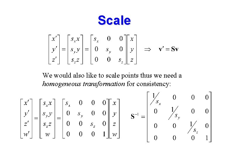
Scale We would also like to scale points thus we need a homogeneous transformation for consistency:

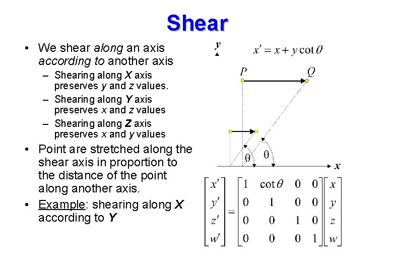
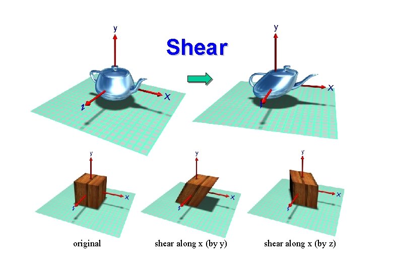
Shear • We shear along an axis according to another axis – Shearing along X axis preserves y and z values. – Shearing along Y axis preserves x and z values – Shearing along Z axis preserves x and y values • Point are stretched along the shear axis in proportion to the distance of the point along another axis. • Example: shearing along X according to Y

Shear original shear along x (by y) shear along x (by z)

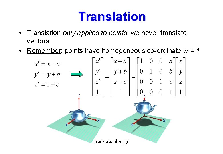
Translation • Translation only applies to points, we never translate vectors. • Remember: points have homogeneous co-ordinate w = 1 translate along y

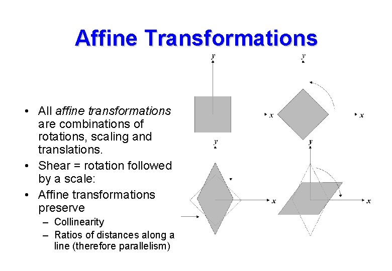
Affine Transformations • All affine transformations are combinations of rotations, scaling and translations. • Shear = rotation followed by a scale: • Affine transformations preserve – Collinearity – Ratios of distances along a line (therefore parallelism)

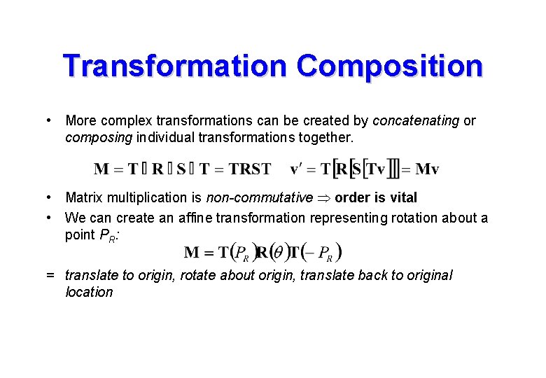
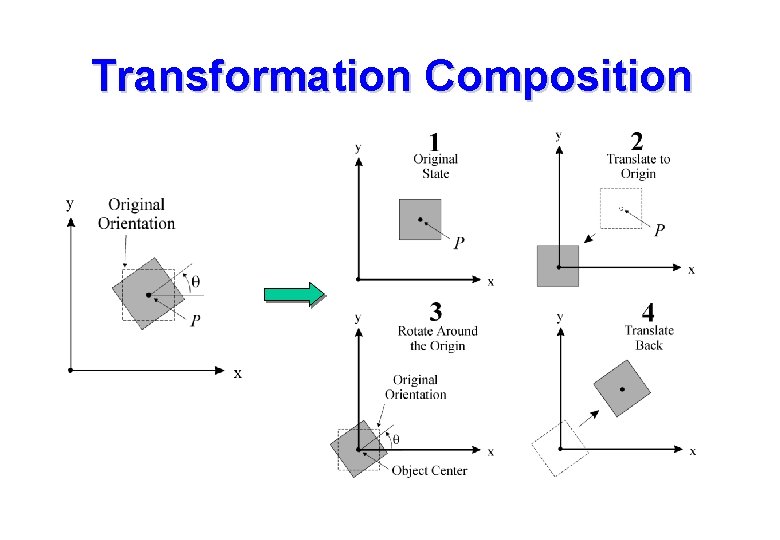
Transformation Composition • More complex transformations can be created by concatenating or composing individual transformations together. • Matrix multiplication is non-commutative order is vital • We can create an affine transformation representing rotation about a point PR: = translate to origin, rotate about origin, translate back to original location

Transformation Composition

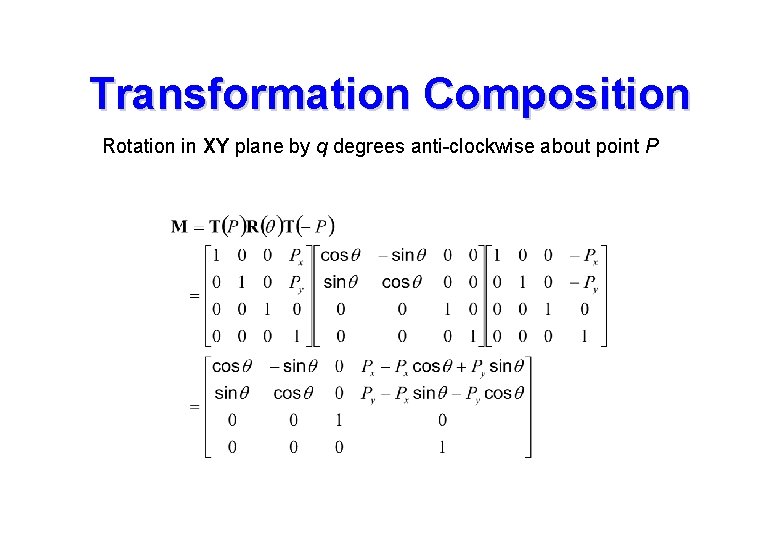
Transformation Composition Rotation in XY plane by q degrees anti-clockwise about point P

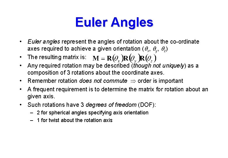
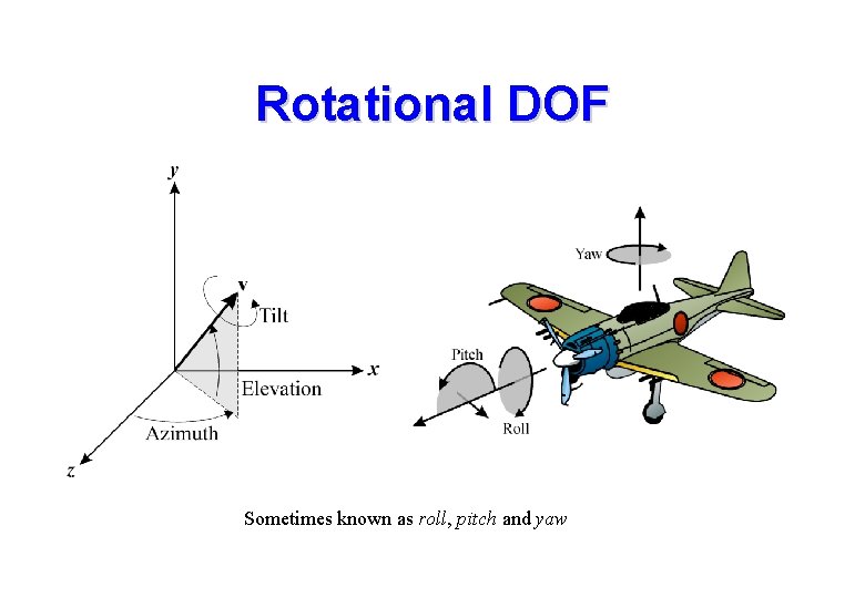
Euler Angles • Euler angles represent the angles of rotation about the co-ordinate axes required to achieve a given orientation (qx, qy, qz) • The resulting matrix is: • Any required rotation may be described (though not uniquely) as a composition of 3 rotations about the coordinate axes. • Remember rotation does not commute order is important • A frequent requirement is to determine the matrix for rotation about an given axis. • Such rotations have 3 degrees of freedom (DOF): – 2 for spherical angles specifying axis orientation – 1 for twist about the rotation axis

Rotational DOF Sometimes known as roll, pitch and yaw

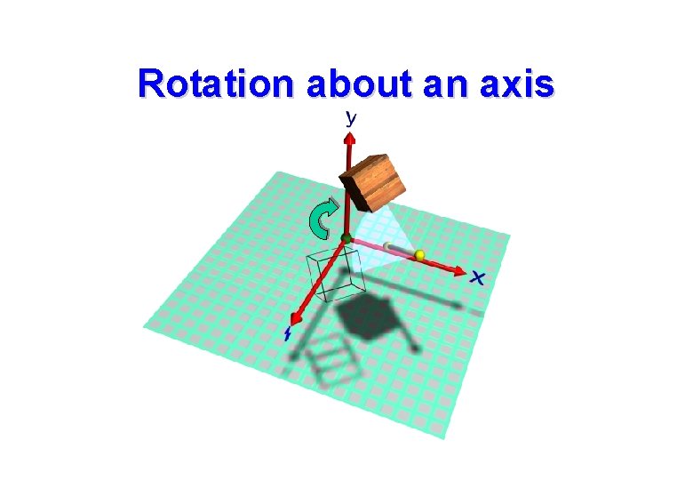
Rotation about an axis

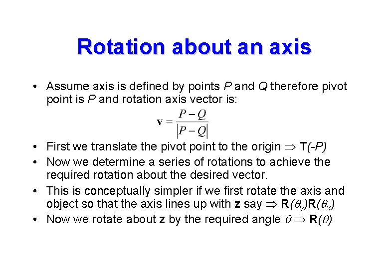
Rotation about an axis • Assume axis is defined by points P and Q therefore pivot point is P and rotation axis vector is: • First we translate the pivot point to the origin T(-P) • Now we determine a series of rotations to achieve the required rotation about the desired vector. • This is conceptually simpler if we first rotate the axis and object so that the axis lines up with z say R(qy)R(qx) • Now we rotate about z by the required angle q R(q)

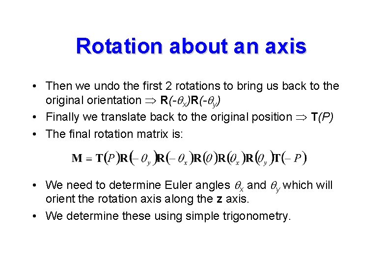
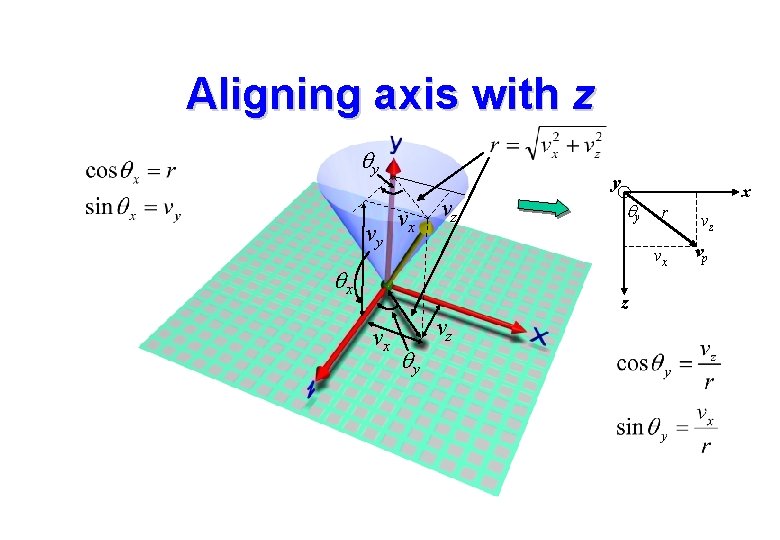
Rotation about an axis • Then we undo the first 2 rotations to bring us back to the original orientation R(-qx)R(-qy) • Finally we translate back to the original position T(P) • The final rotation matrix is: • We need to determine Euler angles qx and qy which will orient the rotation axis along the z axis. • We determine these using simple trigonometry.

Aligning axis with z qy vy y vx vz qx qy z vx qy vz x r vz vx vp

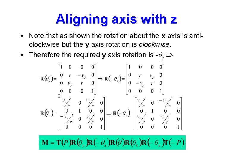
Aligning axis with z • Note that as shown the rotation about the x axis is anticlockwise but the y axis rotation is clockwise. • Therefore the required y axis rotation is -qy

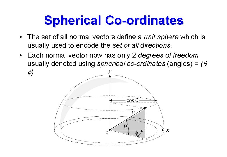
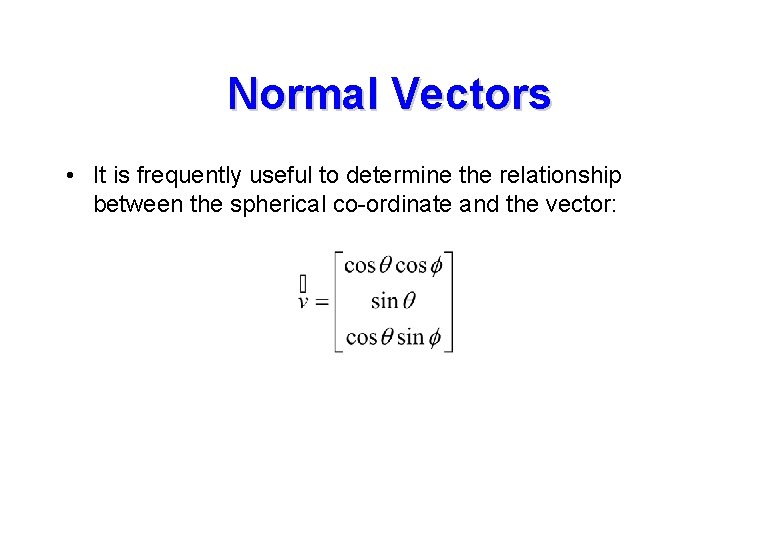
Spherical Co-ordinates • The set of all normal vectors define a unit sphere which is usually used to encode the set of all directions. • Each normal vector now has only 2 degrees of freedom usually denoted using spherical co-ordinates (angles) = (q, f)

Normal Vectors • It is frequently useful to determine the relationship between the spherical co-ordinate and the vector:

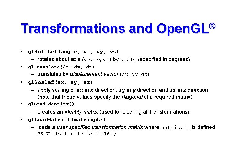
Transformations and Open. GL® • gl. Rotatef(angle, vx, vy, vz) – rotates about axis (vx, vy, vz) by angle (specified in degrees) • gl. Translate(dx, dy, dz) – translates by displacement vector (dx, dy, dz) • gl. Scalef(sx, sy, sz) – apply scaling of sx in x direction, sy in y direction and sz in z direction (note that these values specify the diagonal of a required matrix) • gl. Load. Identity() – creates an identity matrix (used for clearing all transformations) • gl. Load. Matrixf(matrixptr) – loads a user specified transformation matrix where matrixptr is defined as GLfloat matrixptr[16];

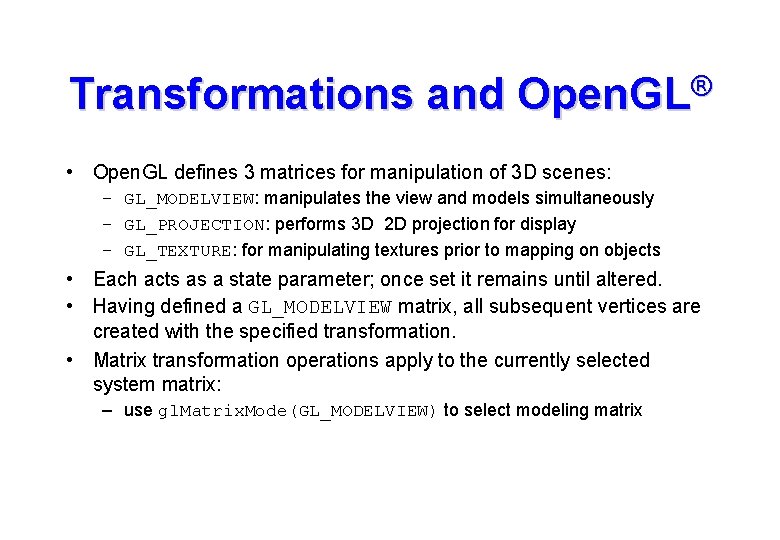
Transformations and Open. GL® • Open. GL defines 3 matrices for manipulation of 3 D scenes: – GL_MODELVIEW: manipulates the view and models simultaneously – GL_PROJECTION: performs 3 D 2 D projection for display – GL_TEXTURE: for manipulating textures prior to mapping on objects • Each acts as a state parameter; once set it remains until altered. • Having defined a GL_MODELVIEW matrix, all subsequent vertices are created with the specified transformation. • Matrix transformation operations apply to the currently selected system matrix: – use gl. Matrix. Mode(GL_MODELVIEW) to select modeling matrix

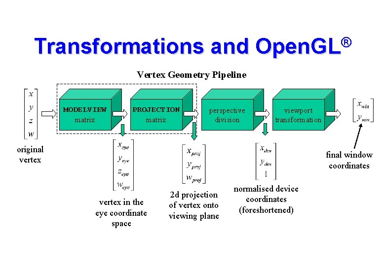
Transformations and Open. GL® Vertex Geometry Pipeline MODELVIEW matrix PROJECTION matrix perspective division viewport transformation original vertex final window coordinates vertex in the eye coordinate space 2 d projection of vertex onto viewing plane normalised device coordinates (foreshortened)

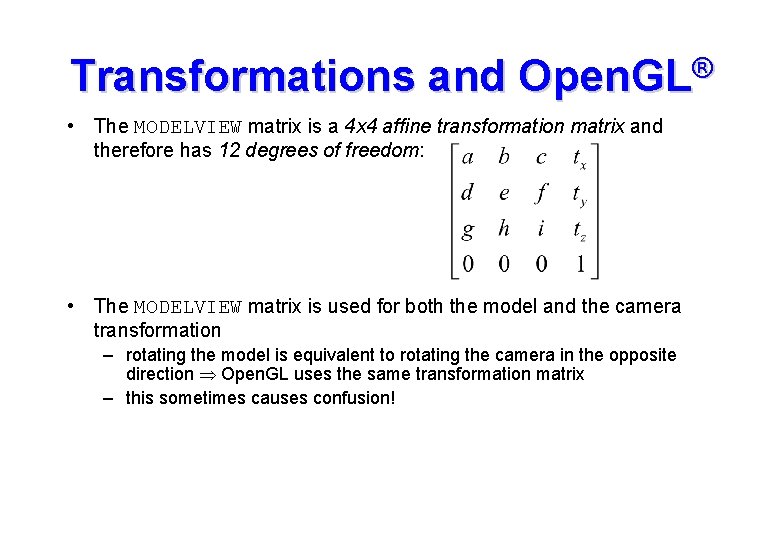
Transformations and Open. GL® • The MODELVIEW matrix is a 4 x 4 affine transformation matrix and therefore has 12 degrees of freedom: • The MODELVIEW matrix is used for both the model and the camera transformation – rotating the model is equivalent to rotating the camera in the opposite direction Open. GL uses the same transformation matrix – this sometimes causes confusion!

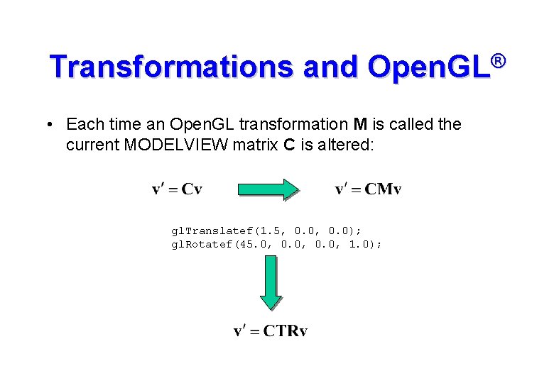
Transformations and Open. GL® • Each time an Open. GL transformation M is called the current MODELVIEW matrix C is altered: gl. Translatef(1. 5, 0. 0); gl. Rotatef(45. 0, 0. 0, 1. 0);

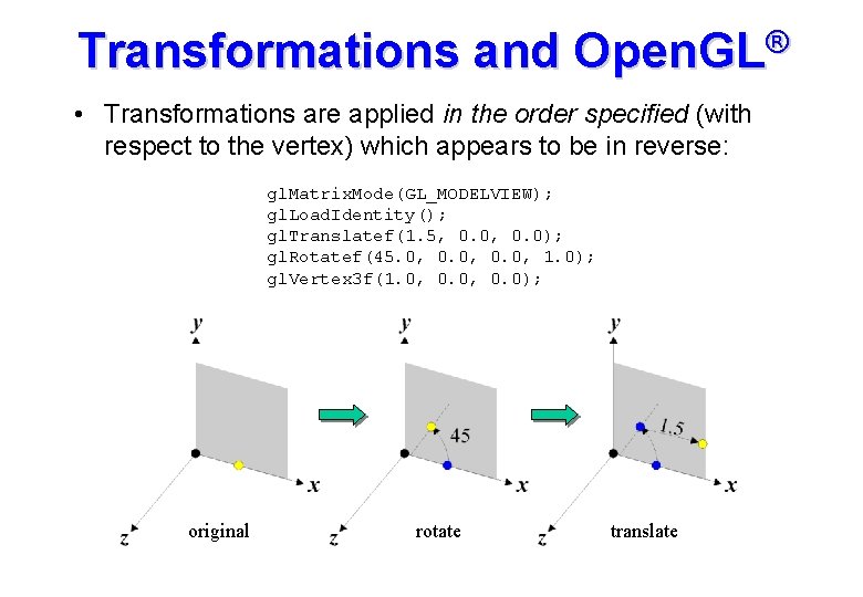
Transformations and Open. GL® • Transformations are applied in the order specified (with respect to the vertex) which appears to be in reverse: gl. Matrix. Mode(GL_MODELVIEW); gl. Load. Identity(); gl. Translatef(1. 5, 0. 0); gl. Rotatef(45. 0, 0. 0, 1. 0); gl. Vertex 3 f(1. 0, 0. 0); original rotate translate

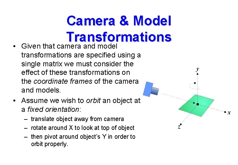
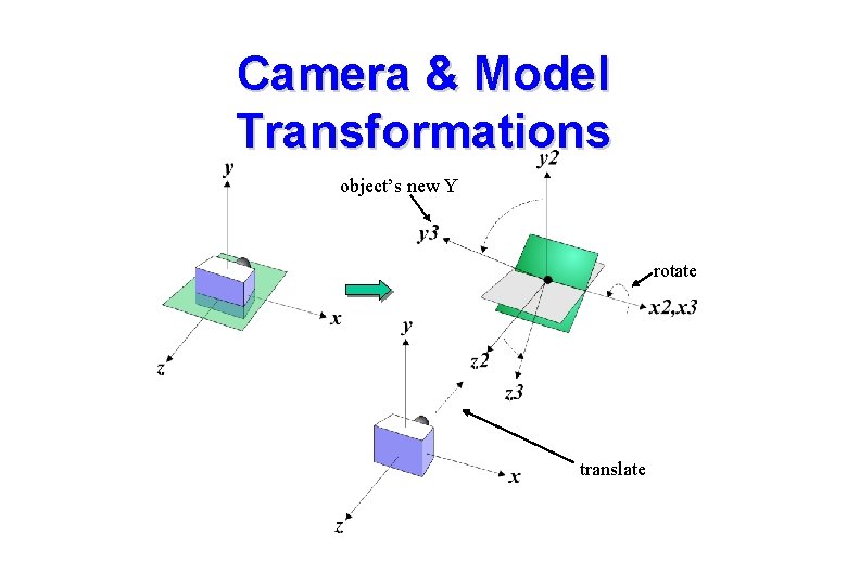
• Camera & Model Transformations Given that camera and model transformations are specified using a single matrix we must consider the effect of these transformations on the coordinate frames of the camera and models. • Assume we wish to orbit an object at a fixed orientation: – translate object away from camera – rotate around X to look at top of object – then pivot around object’s Y in order to orbit properly.

Camera & Model Transformations • If the GL_MODELVIEW matrix is an identity matrix then the camera frame and the model frame are the same. – i. e. they are specified using the same co-ordinate system • If we issue command gl. Translatef(0. 0, -10. 0) and then create the model: – a vertex at [0, 0, 0] in the model will be at [0, 0, -10] in the camera frame – i. e. we have moved the object away from the camera • This may be viewed conceptually in 2 ways: – we have positioned the object with respect to the world frame – we have moved the world-frame with respect to the camera frame

Camera & Model Transformations object’s new Y rotate translate

Camera & Model Transformations • A “local frame view” is usually adopted as it extends naturally to the specification of hierarchical model frames. • This allows creation of jointed assemblies – articulated figures (animals, robots etc. ) • In the hierarchical model, each sub-component has its own local frame. • Changes made to the parent frame are propagated down to the child frames (thus all models in a branch are globally controlled by the parent). • This simplifies the specification of animation.

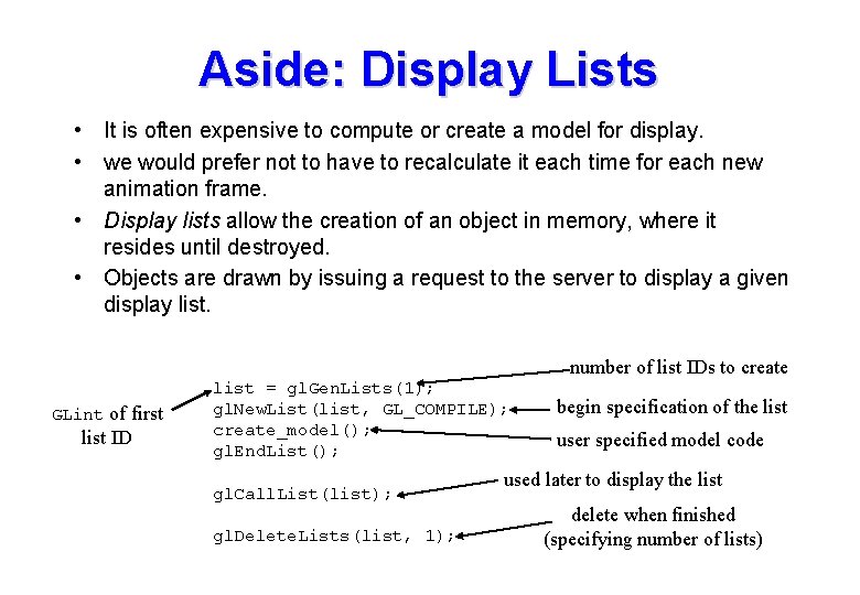
Aside: Display Lists • It is often expensive to compute or create a model for display. • we would prefer not to have to recalculate it each time for each new animation frame. • Display lists allow the creation of an object in memory, where it resides until destroyed. • Objects are drawn by issuing a request to the server to display a given display list. number of list IDs to create GLint of first list ID list = gl. Gen. Lists(1); gl. New. List(list, GL_COMPILE); create_model(); gl. End. List(); gl. Call. List(list); gl. Delete. Lists(list, 1); begin specification of the list user specified model code used later to display the list delete when finished (specifying number of lists)

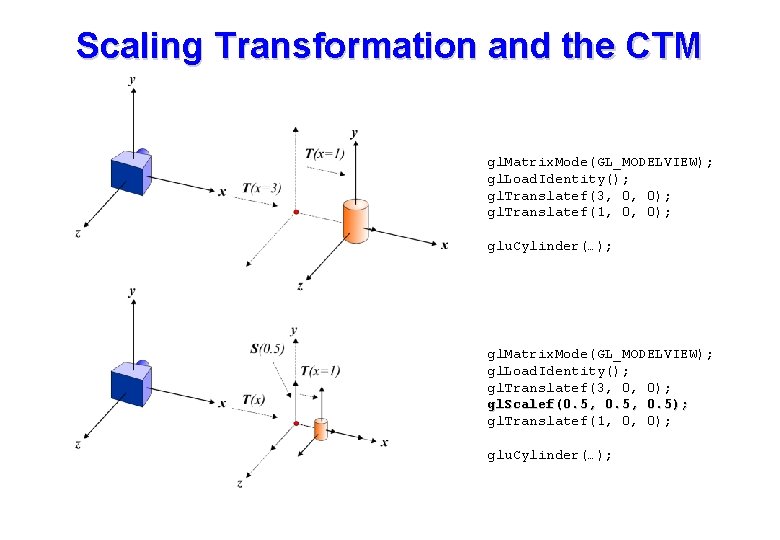
Model Transformations • As the MODELVIEW matrix is changed objects are created with respect to a changing transformation. • This is often termed the current transformation matrix or CTM. • The CTM behaves like a 3 D pointer, selecting new positions and orientations for the creation of geometries. • The only complication with this view is that each new CTM is derived from a previous CTM, i. e. all CTMs are specified relative to previous versions. • A scaling transformation cause some confusion.

Scaling Transformation and the CTM gl. Matrix. Mode(GL_MODELVIEW); gl. Load. Identity(); gl. Translatef(3, 0, 0); gl. Translatef(1, 0, 0); glu. Cylinder(…); gl. Matrix. Mode(GL_MODELVIEW); gl. Load. Identity(); gl. Translatef(3, 0, 0); gl. Scalef(0. 5, 0. 5); gl. Translatef(1, 0, 0); glu. Cylinder(…);

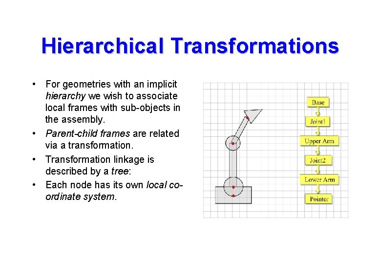
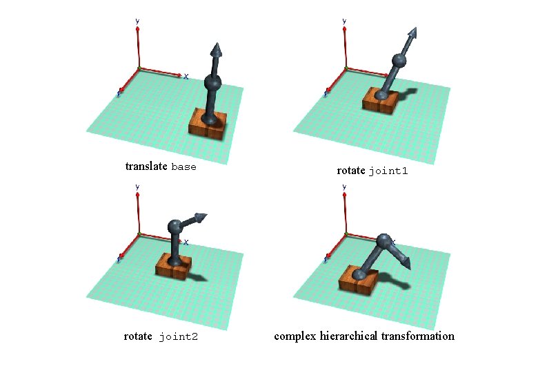
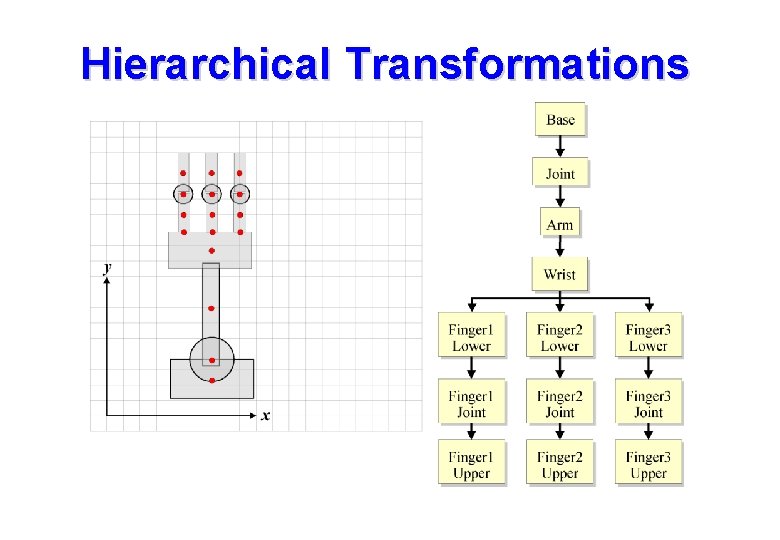
Hierarchical Transformations • For geometries with an implicit hierarchy we wish to associate local frames with sub-objects in the assembly. • Parent-child frames are related via a transformation. • Transformation linkage is described by a tree: • Each node has its own local coordinate system.

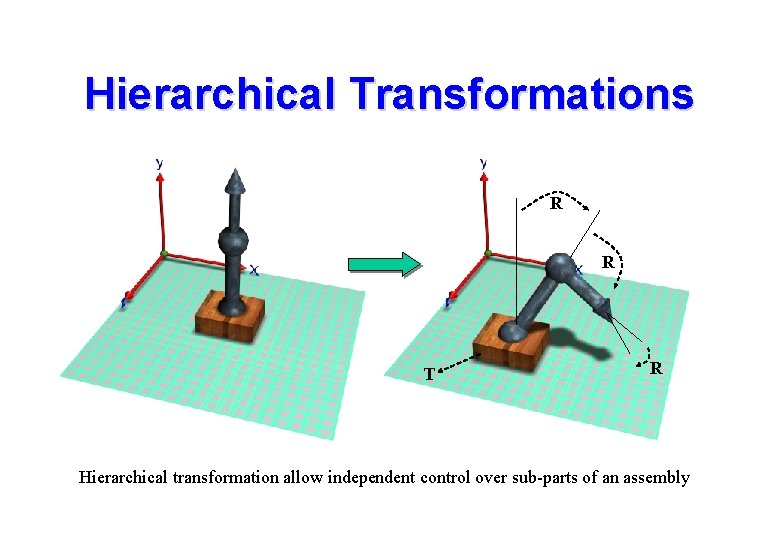
Hierarchical Transformations R R T R Hierarchical transformation allow independent control over sub-parts of an assembly

translate base rotate joint 2 rotate joint 1 complex hierarchical transformation

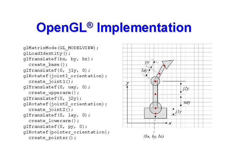
Open. GL® Implementation gl. Matrix. Mode(GL_MODELVIEW); gl. Load. Identity(); gl. Translatef(bx, by, bz); create_base(); gl. Translatef(0, j 1 y, 0); gl. Rotatef(joint 1_orientation); create_joint 1(); gl. Translatef(0, uay, 0); create_upperarm(); gl. Translatef(0, j 2 y); gl. Rotatef(joint 2_orientation); create_joint 2(); gl. Translatef(0, lay, 0); create_lowerarm(); gl. Translatef(0, py, 0); gl. Rotatef(pointer_orientation); create_pointer();

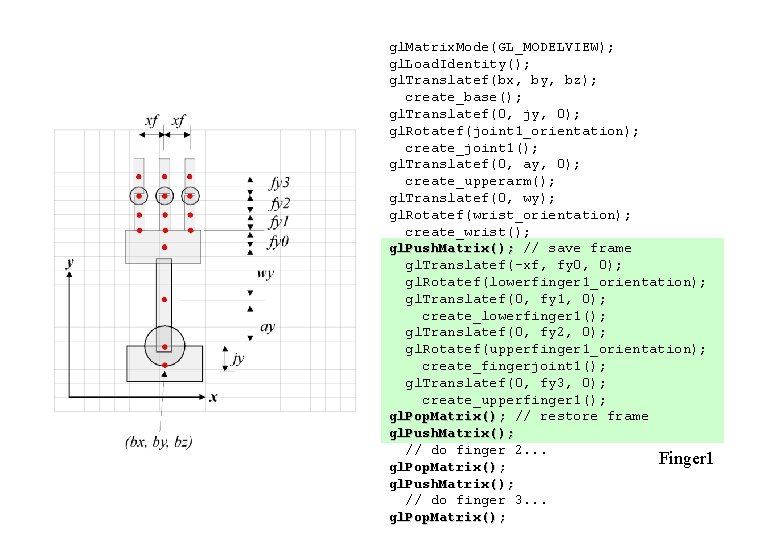
Hierarchical Transformations • The previous example had simple one-to-one parent-child linkages. • In general there may be many child frames derived from a single parent frame. • we need some mechanism to remember the parent frame and return to it when creating new children. • Open. GL provide a matrix stack for just this purpose: – gl. Push. Matrix() saves the CTM – gl. Pop. Matrix() returns to the last saved CTM

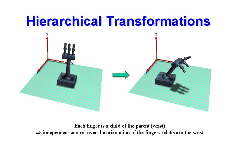
Hierarchical Transformations Each finger is a child of the parent (wrist) independent control over the orientation of the fingers relative to the wrist

Hierarchical Transformations

gl. Matrix. Mode(GL_MODELVIEW); gl. Load. Identity(); gl. Translatef(bx, by, bz); create_base(); gl. Translatef(0, jy, 0); gl. Rotatef(joint 1_orientation); create_joint 1(); gl. Translatef(0, ay, 0); create_upperarm(); gl. Translatef(0, wy); gl. Rotatef(wrist_orientation); create_wrist(); gl. Push. Matrix(); // save frame gl. Translatef(-xf, fy 0, 0); gl. Rotatef(lowerfinger 1_orientation); gl. Translatef(0, fy 1, 0); create_lowerfinger 1(); gl. Translatef(0, fy 2, 0); gl. Rotatef(upperfinger 1_orientation); create_fingerjoint 1(); gl. Translatef(0, fy 3, 0); create_upperfinger 1(); gl. Pop. Matrix(); // restore frame gl. Push. Matrix(); // do finger 2. . . Finger 1 gl. Pop. Matrix(); gl. Push. Matrix(); // do finger 3. . . gl. Pop. Matrix();

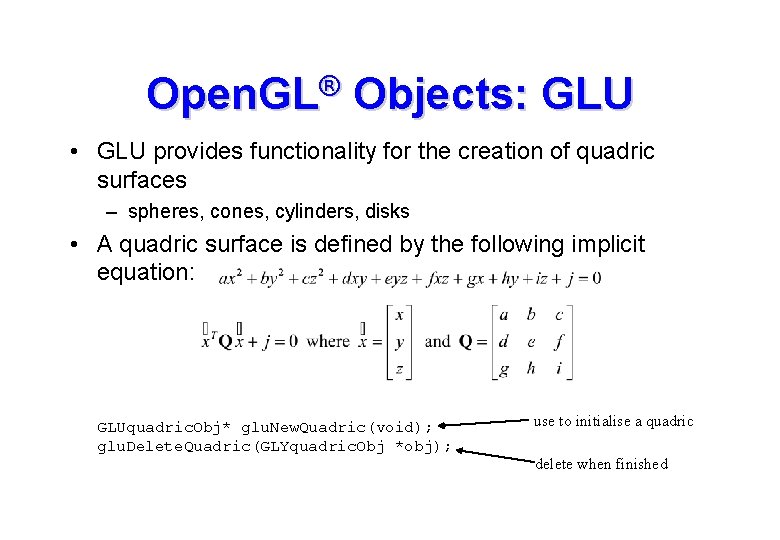
Open. GL® Objects: GLU • GLU provides functionality for the creation of quadric surfaces – spheres, cones, cylinders, disks • A quadric surface is defined by the following implicit equation: GLUquadric. Obj* glu. New. Quadric(void); glu. Delete. Quadric(GLYquadric. Obj *obj); use to initialise a quadric delete when finished

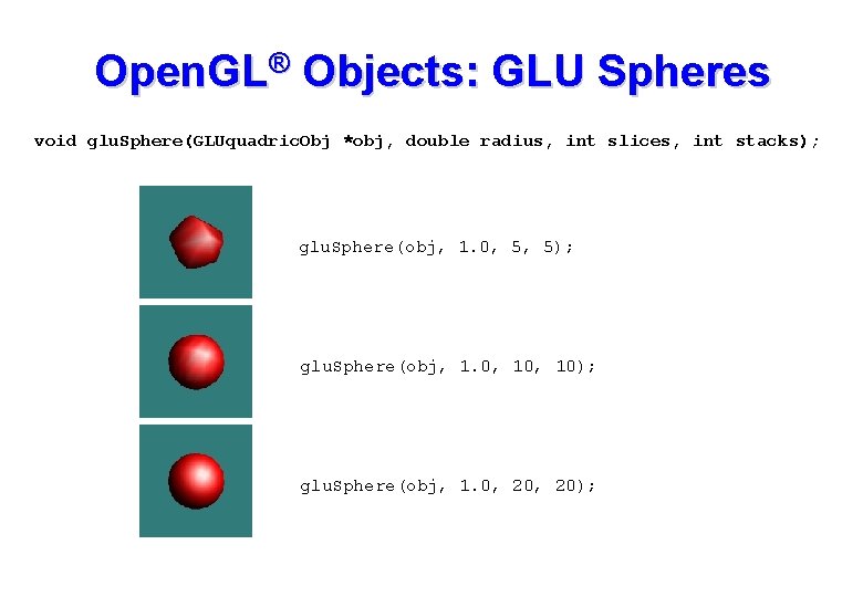
Open. GL® Objects: GLU Spheres void glu. Sphere(GLUquadric. Obj *obj, double radius, int slices, int stacks); glu. Sphere(obj, 1. 0, 5, 5); glu. Sphere(obj, 1. 0, 10); glu. Sphere(obj, 1. 0, 20);

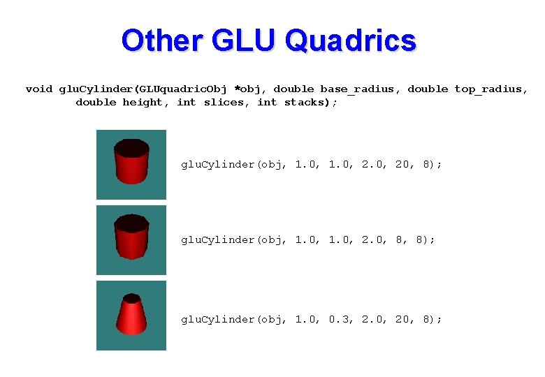
Other GLU Quadrics void glu. Cylinder(GLUquadric. Obj *obj, double base_radius, double top_radius, double height, int slices, int stacks); glu. Cylinder(obj, 1. 0, 20, 8); glu. Cylinder(obj, 1. 0, 2. 0, 8, 8); glu. Cylinder(obj, 1. 0, 0. 3, 2. 0, 20, 8);

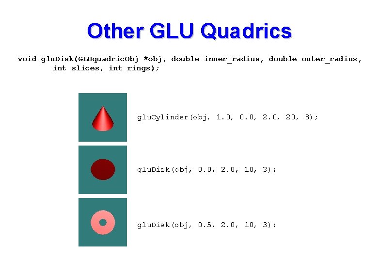
Other GLU Quadrics void glu. Disk(GLUquadric. Obj *obj, double inner_radius, double outer_radius, int slices, int rings); glu. Cylinder(obj, 1. 0, 0. 0, 20, 8); glu. Disk(obj, 0. 0, 2. 0, 10, 3); glu. Disk(obj, 0. 5, 2. 0, 10, 3);

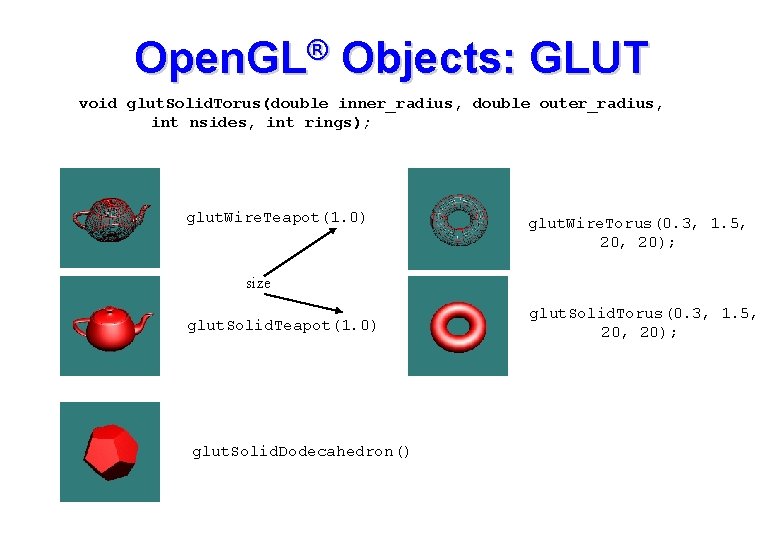
Open. GL® Objects: GLUT void glut. Solid. Torus(double inner_radius, double outer_radius, int nsides, int rings); glut. Wire. Teapot(1. 0) glut. Wire. Torus(0. 3, 1. 5, 20); size glut. Solid. Teapot(1. 0) glut. Solid. Dodecahedron() glut. Solid. Torus(0. 3, 1. 5, 20);