Transformations What are they and How to do

Transformations What are they and How to do them George Silvis SGEO 10/2019 AAVSO meeting at Las Cruces

• We’re an association of observers • We need to be able share data by submitting it to the AID, the AAVSO International Database • Which means the data must be comparable • We do this by the process of “standardization”

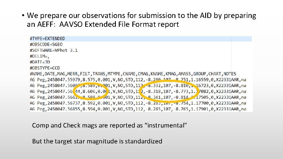
• We prepare our observations for submission to the AID by preparing an AEFF: AAVSO Extended File Format report Comp and Check mags are reported as “instrumental” But the target star magnitude is standardized

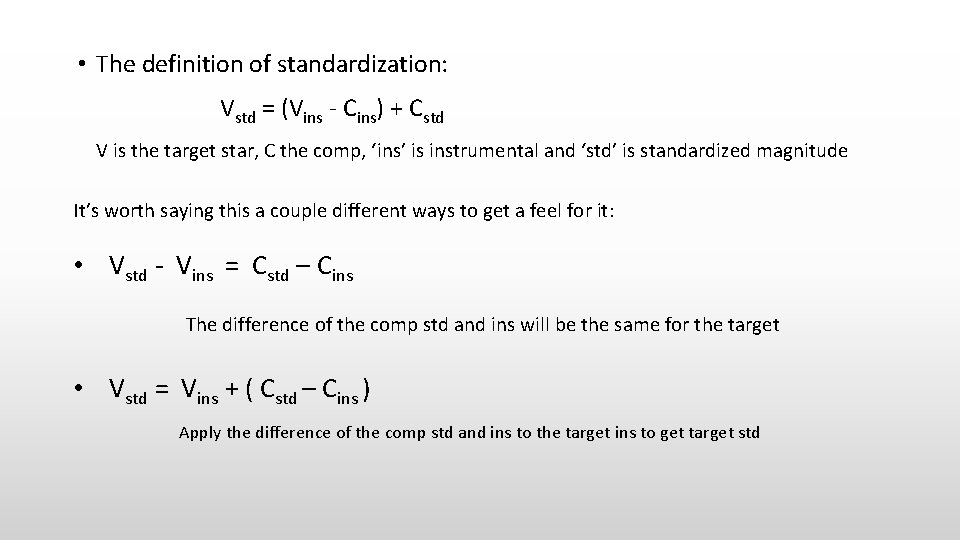
• The definition of standardization: Vstd = (Vins - Cins) + Cstd V is the target star, C the comp, ‘ins’ is instrumental and ‘std’ is standardized magnitude It’s worth saying this a couple different ways to get a feel for it: • Vstd - Vins = Cstd – Cins The difference of the comp std and ins will be the same for the target • Vstd = Vins + ( Cstd – Cins ) Apply the difference of the comp std and ins to the target ins to get target std

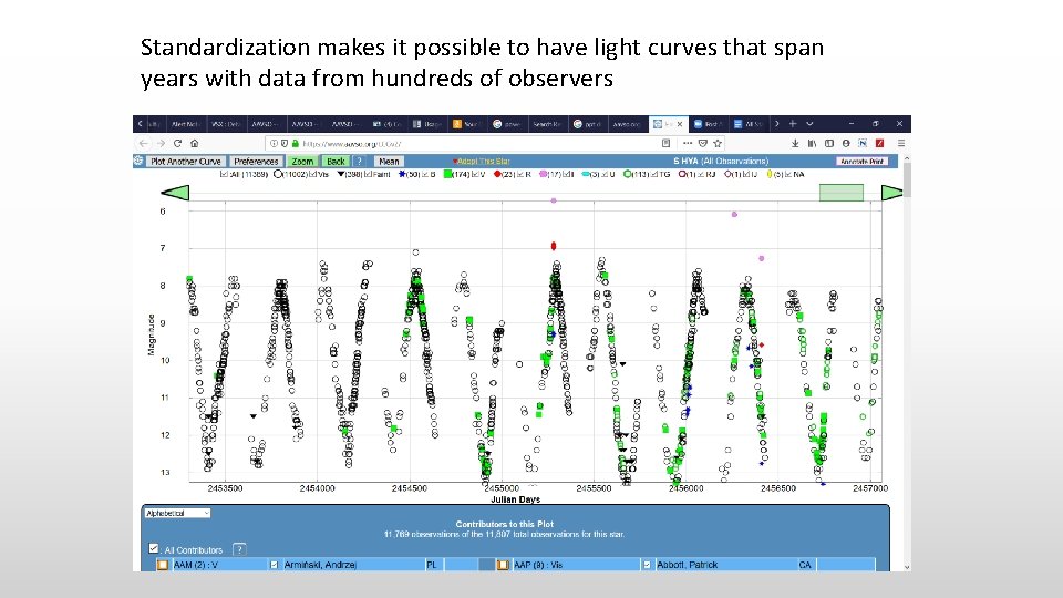
Standardization makes it possible to have light curves that span years with data from hundreds of observers

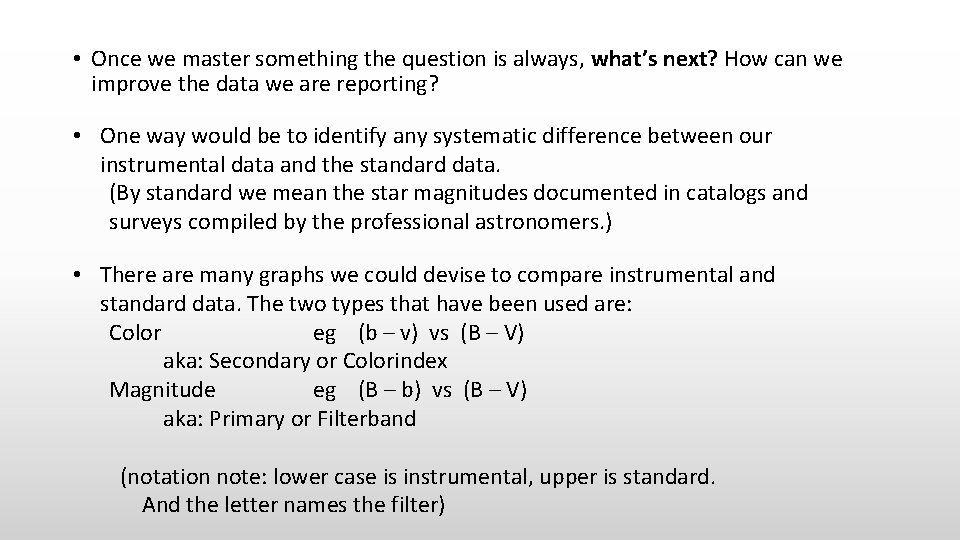
• Once we master something the question is always, what’s next? How can we improve the data we are reporting? • One way would be to identify any systematic difference between our instrumental data and the standard data. (By standard we mean the star magnitudes documented in catalogs and surveys compiled by the professional astronomers. ) • There are many graphs we could devise to compare instrumental and standard data. The two types that have been used are: Color eg (b – v) vs (B – V) aka: Secondary or Colorindex Magnitude eg (B – b) vs (B – V) aka: Primary or Filterband (notation note: lower case is instrumental, upper is standard. And the letter names the filter)

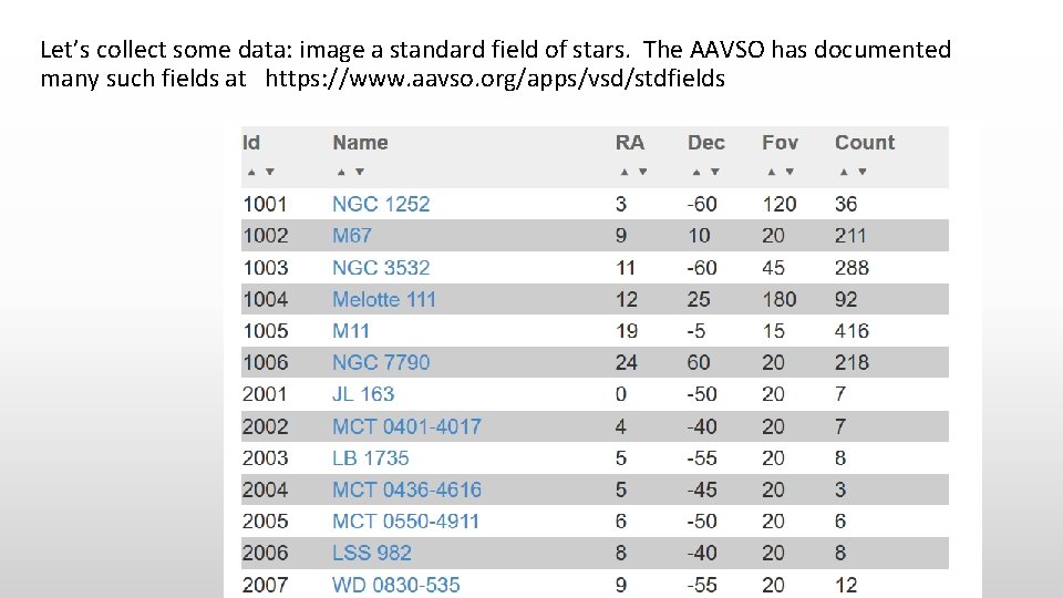
Let’s collect some data: image a standard field of stars. The AAVSO has documented many such fields at https: //www. aavso. org/apps/vsd/stdfields

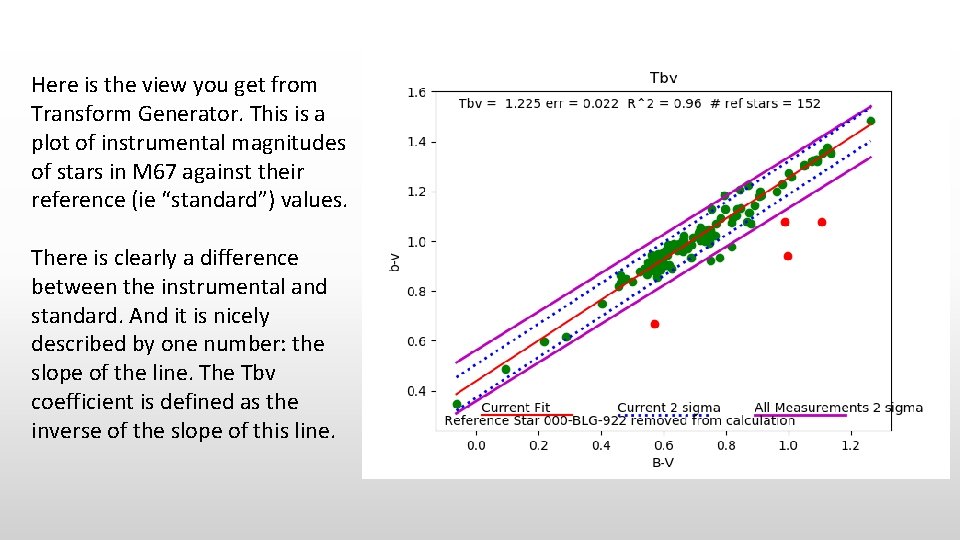
Here is the view you get from Transform Generator. This is a plot of instrumental magnitudes of stars in M 67 against their reference (ie “standard”) values. There is clearly a difference between the instrumental and standard. And it is nicely described by one number: the slope of the line. The Tbv coefficient is defined as the inverse of the slope of this line.

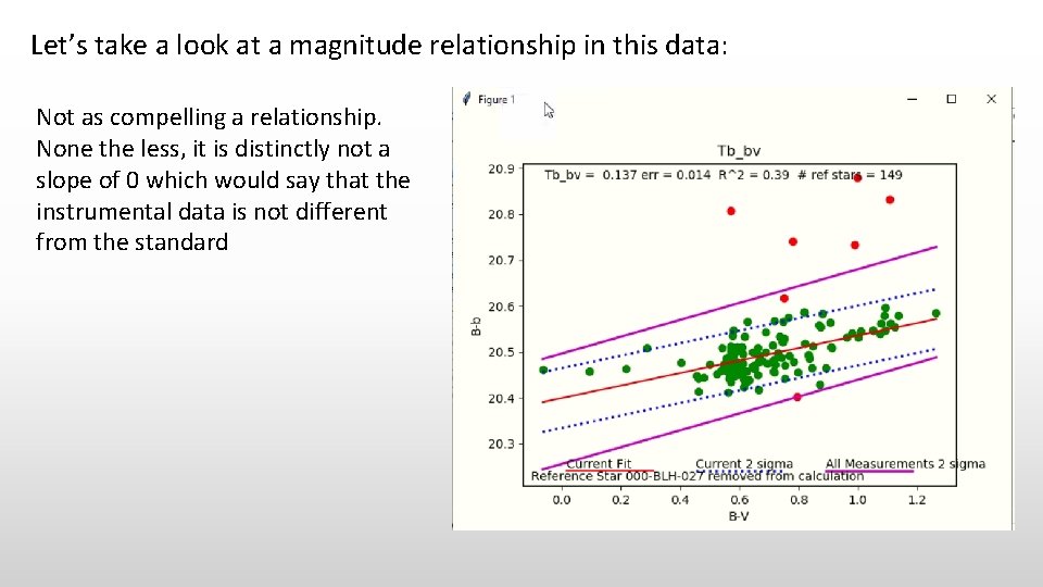
Let’s take a look at a magnitude relationship in this data: Not as compelling a relationship. None the less, it is distinctly not a slope of 0 which would say that the instrumental data is not different from the standard

If we can draw these graphs and reproduce the results with multiple sets of standard field images, then we know our system (our scope, filters, camera) are different from the Standard. How can we use this knowledge to correct our data so that when it goes into the AID we are reporting our best understanding of standard data? This process of applying the knowledge of our systems difference from the standard to our data to remove that system bias is what we call “Transformation”

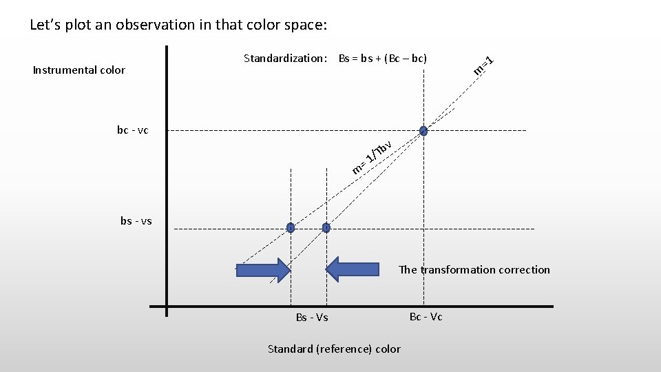
Let’s plot an observation in that color space: Instrumental color Standardization: Bs = bs + (Bc – bc) m =1 bc - vc v = m Tb / 1 bs - vs The transformation correction Bs - Vs Standard (reference) color Bc - Vc

How do we use this graph to compute Bs or Vs? Simply take the definition of Tbv: 1 / Tbv = ((bs-vs)-(bc-vc)) / ((Bs-Vs)-(Bc-Vc)) And rearrange to bring the variable you want out to the left: Bs = Vs + (Bc-Vc) + Tbv* ((bs-vs)-(bc-vc)) Or we could use Tb_bv: Tb_bv = ((Bs-bs)-(Bc-bc)) / ((Bs-Vs)-(Bc-Vc)) to get: Bs = bs + (Bc-bc) + Tb_bv * ((Bs-Vs)-(Bc-Vc)) nota bene: It is not necessary to isolate the Bs variable to the left!

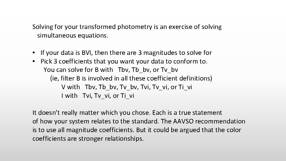
Solving for your transformed photometry is an exercise of solving simultaneous equations. • If your data is BVI, then there are 3 magnitudes to solve for • Pick 3 coefficients that you want your data to conform to. You can solve for B with Tbv, Tb_bv, or Tv_bv (ie, filter B is involved in all these coefficient definitions) V with Tbv, Tb_bv, Tvi, Tv_vi, or Ti_vi I with Tvi, Tv_vi, or Ti_vi It doesn’t really matter which you chose. Each is a true statement of how your system relates to the standard. The AAVSO recommendation is to use all magnitude coefficients. But it could be argued that the color coefficients are stronger relationships.

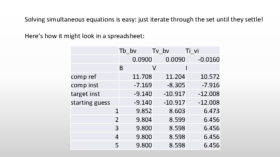
Solving simultaneous equations is easy: just iterate through the set until they settle! Here’s how it might look in a spreadsheet: Tb_bv Tv_bv Ti_vi 0. 0900 0. 0090 -0. 0160 B V I comp ref 11. 708 11. 204 10. 572 comp inst -7. 169 -8. 305 -7. 916 target inst -9. 140 -10. 917 -12. 008 starting guess -9. 140 -10. 917 -12. 008 1 9. 852 8. 603 6. 473 2 9. 804 8. 599 6. 456 3 9. 800 8. 598 6. 456 4 9. 800 8. 598 6. 456 5 9. 800 8. 598 6. 456

The charm of this method is • It extends to multifilter systems; UBVRI is a snap • And you can experiment with more complex constraints; Maybe the b-v vs B-V relationship is not a line, but a curve… • Other presentations of the transformation process drown you in algebraic gymnastics

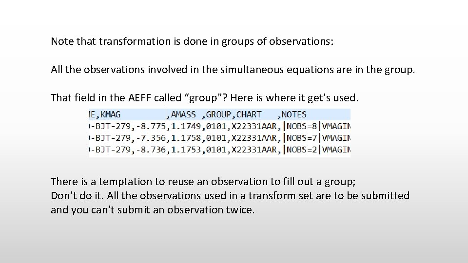
Note that transformation is done in groups of observations: All the observations involved in the simultaneous equations are in the group. That field in the AEFF called “group”? Here is where it get’s used. There is a temptation to reuse an observation to fill out a group; Don’t do it. All the observations used in a transform set are to be submitted and you can’t submit an observation twice.

Take aways: • Each coefficient is a truth about how your system relates to the standard • Each coefficient implies an equation • Using iteration it is easy to solve these sets of simultaneous equations

Here we have been using transformation to remove your system idiosyncrasies from your data. But this process can also be used to bridge filter set definitions. . A DSLR camera reports with filters TB, TG and TR. If you have created a set of coefficients for your camera, the transformation process results in data in the filters of the standards, B V and R. There are limits to how far apart the filters can be to bridge. TR to R is a bit of a stretch.

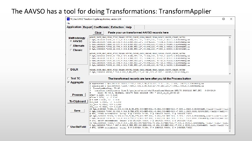
The AAVSO has a tool for doing Transformations: Transform. Applier

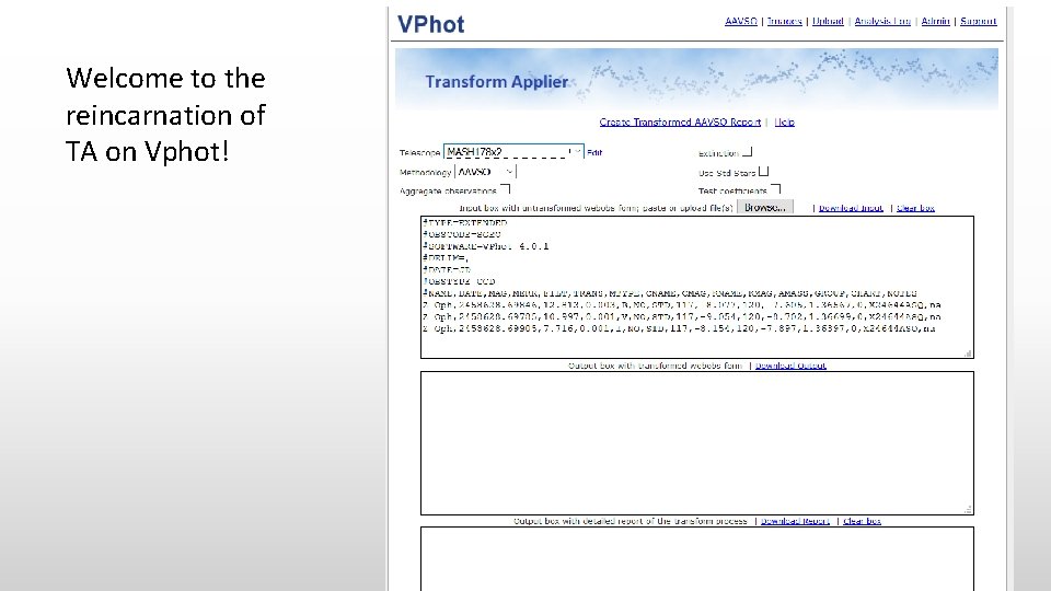
Welcome to the reincarnation of TA on Vphot!

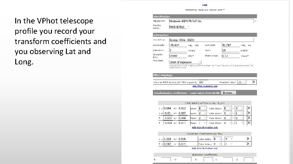
In the VPhot telescope profile you record your transform coefficients and you observing Lat and Long.

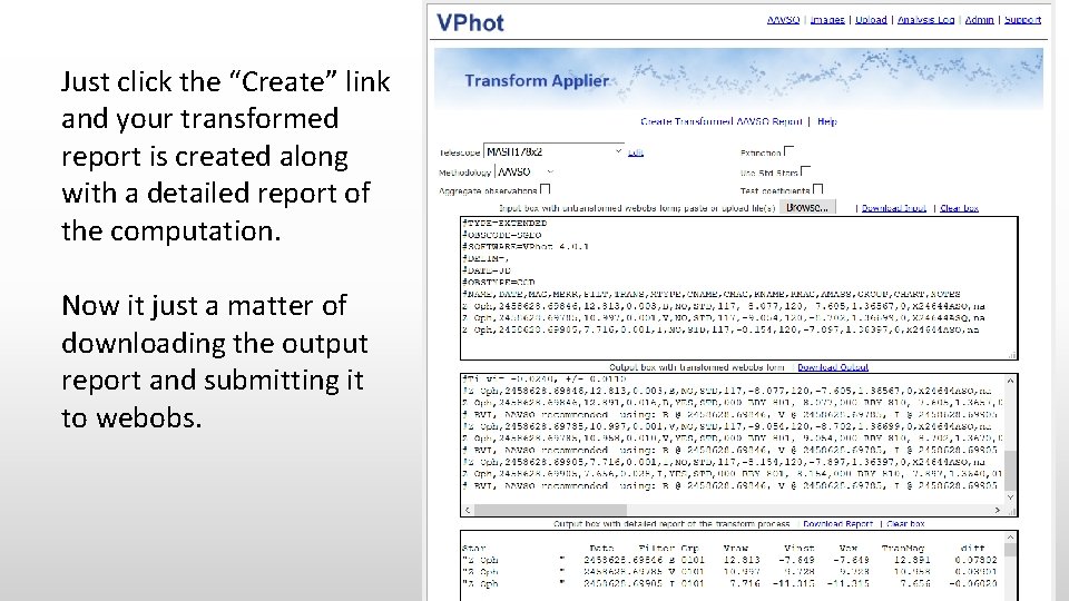
Just click the “Create” link and your transformed report is created along with a detailed report of the computation. Now it just a matter of downloading the output report and submitting it to webobs.

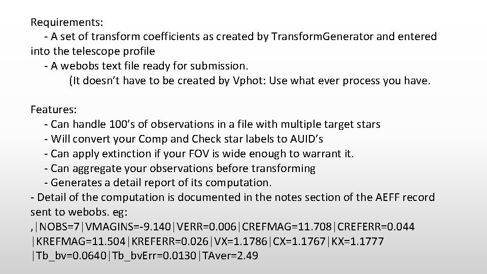
Requirements: - A set of transform coefficients as created by Transform. Generator and entered into the telescope profile - A webobs text file ready for submission. (It doesn’t have to be created by Vphot: Use what ever process you have. Features: - Can handle 100’s of observations in a file with multiple target stars - Will convert your Comp and Check star labels to AUID’s - Can apply extinction if your FOV is wide enough to warrant it. - Can aggregate your observations before transforming - Generates a detail report of its computation. - Detail of the computation is documented in the notes section of the AEFF record sent to webobs. eg: , |NOBS=7|VMAGINS=-9. 140|VERR=0. 006|CREFMAG=11. 708|CREFERR=0. 044 |KREFMAG=11. 504|KREFERR=0. 026|VX=1. 1786|CX=1. 1767|KX=1. 1777 |Tb_bv=0. 0640|Tb_bv. Err=0. 0130|TAver=2. 49

In conclusion • We know what transformation is and what it looks like graphically • We see how it can be computed • And we’ve seen that the AAVSO has tools to help you do it: Transform. Generator, Transform. Applier and now Vphot • So, go forth and transform your data!