Transformations of ContinuousTime Signals Continuous time signal Time


 is periodic if given t and T , is there some")

 is (1/3) as follows")
 is the initial current RC In")
= C eat C and a can be complex Exponential Signals")

")

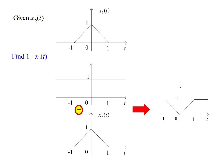
 defined as")
 (2)")

")
 Exercise")
 This property is known as “convolution” which will be useful in")


")


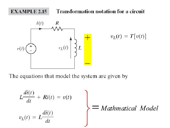
 are expressed as equations")


![Representation of a general system y(t) = T[x(t)] where the notation T[x(t)] indicates a](https://slidetodoc.com/presentation_image/a89970510f7762e28eed0d327118c82a/image-51.jpg "Representation of a general system y(t) = T[x(t)] where the notation T[x(t)] indicates a")

- Slides: 73
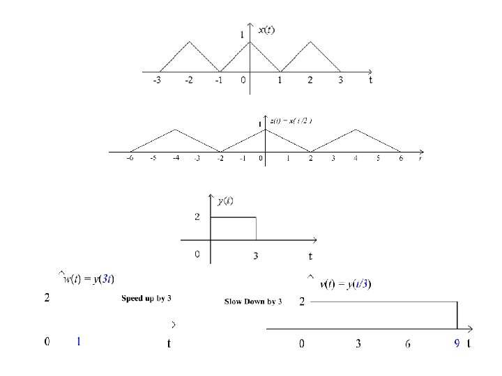
Transformations of Continuous-Time Signals Continuous time signal: • Time is a continuous variable • The signal itself need not be continuous. Time Reversal
Time Reversal compressing Expanding
Let
2. 2
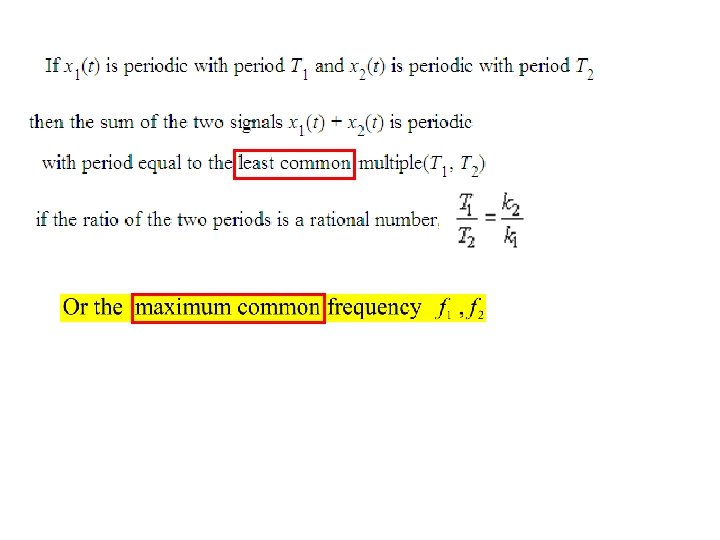
Periodic Functions X(t) is periodic if given t and T , is there some period T > 0 such that
The common frequencies
You can show that the period T 0 of x(t) is (1/3) as follows Since Similarly
2. 3 Common Signals in Engineering RL i(0) is the initial current RC In general Exponential function
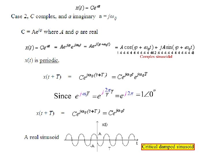
Exponential Signals x(t )= C eat C and a can be complex Exponential Signals appear in the solution of many physical systems Chapter 7 in EE 202 RL and RC Chapter 9 in 202 Sinusoidal steady state Sinusoidal ? What that’s to do with the exponential ? Euler’s identity
Chapter 7 in EE 201 RL and RC
(The most general case)
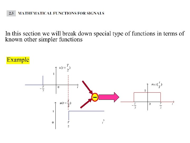
2. 4
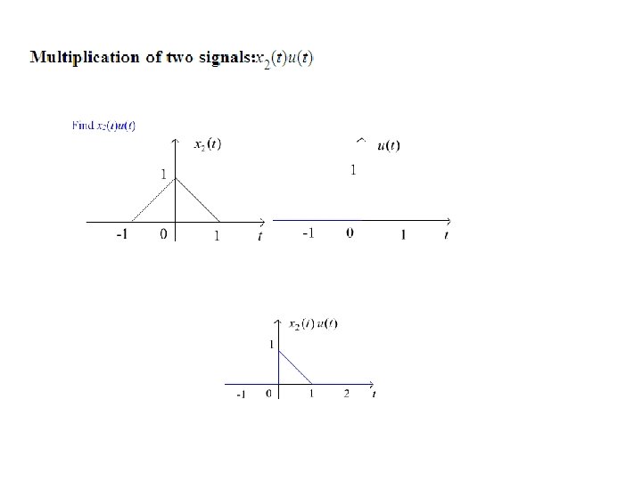
Block function (window) defined as
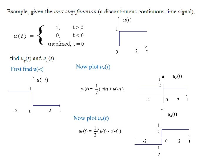
The unit step function has the property (1) (2)
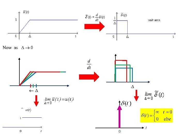
The Unit Impulse Function let's look at a signal What is its derivative ? Define it as :
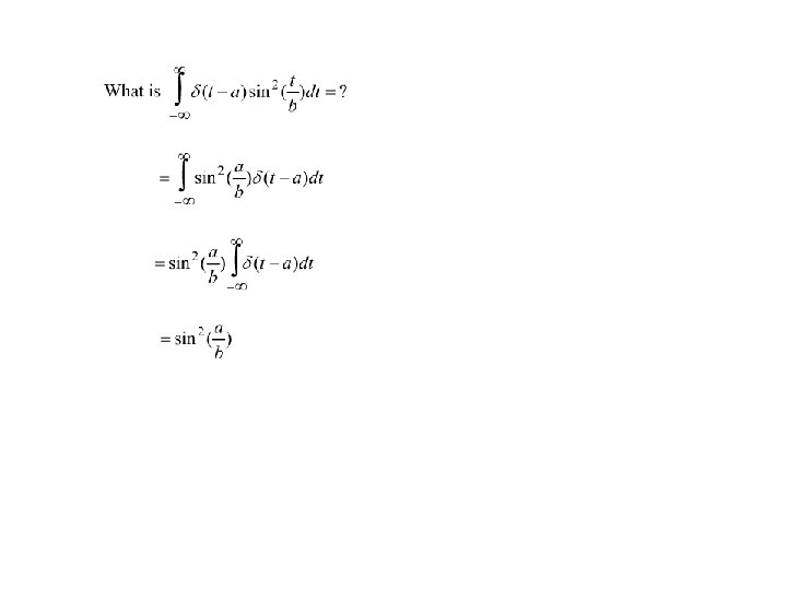
Properties of Delta Function (I)
( II ) Exercise
( II ) This property is known as “convolution” which will be useful in chapter 3
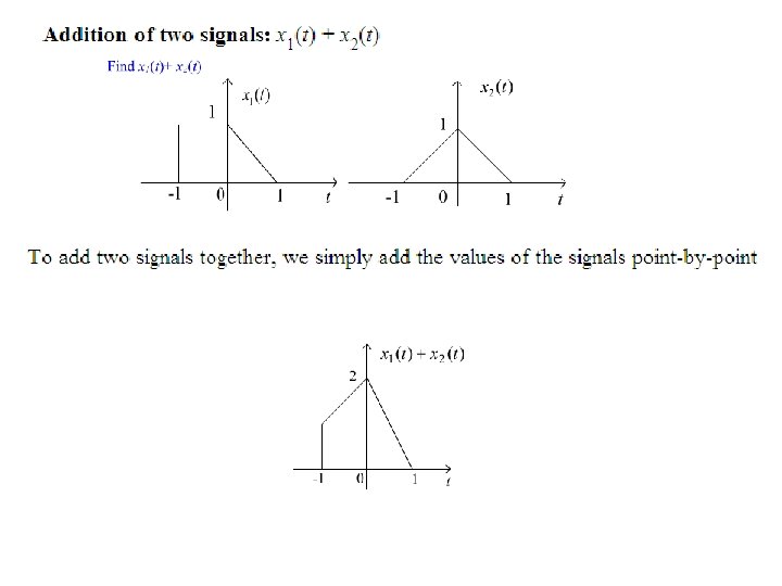
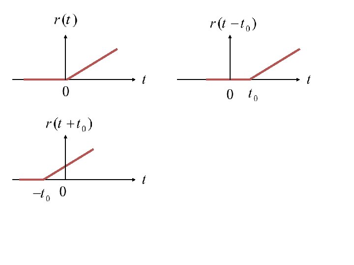
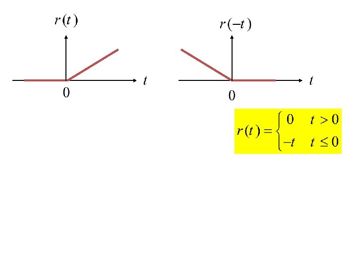
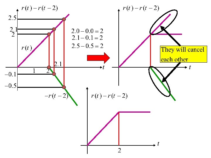
Step Function Ramp Function
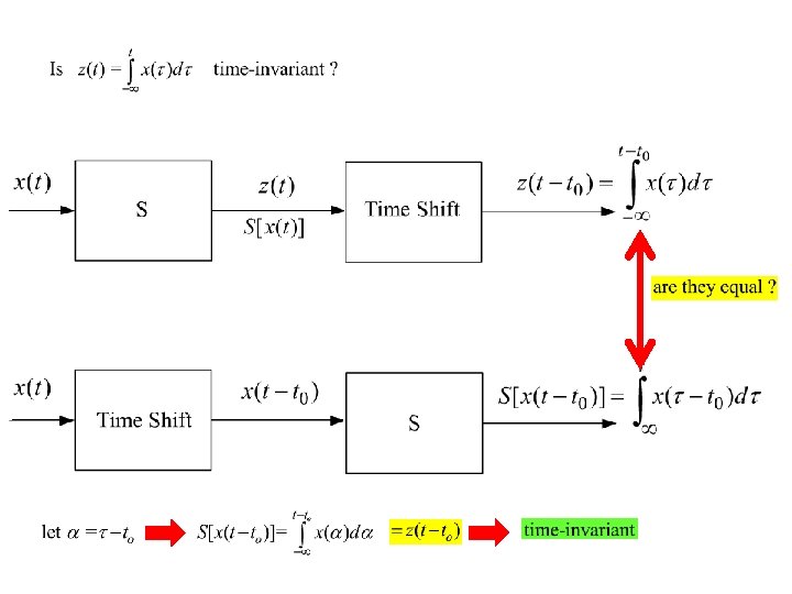
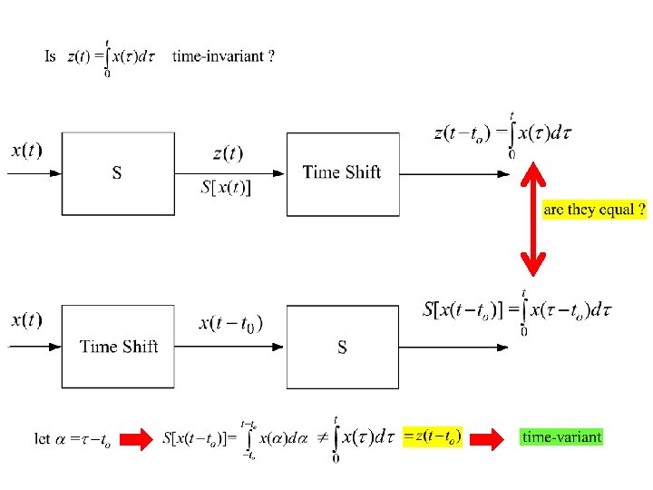
Unit Step Function Integration Unit Ramp Function
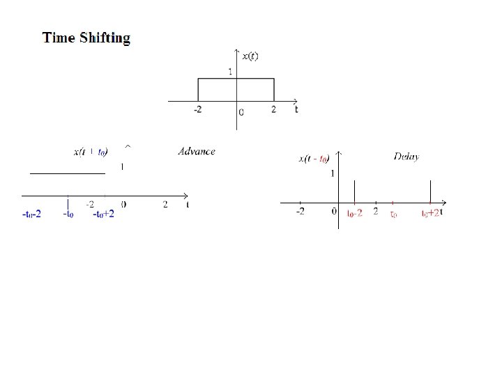
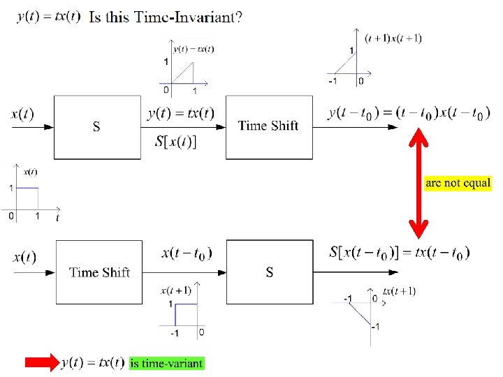
Time Shift
Time folding
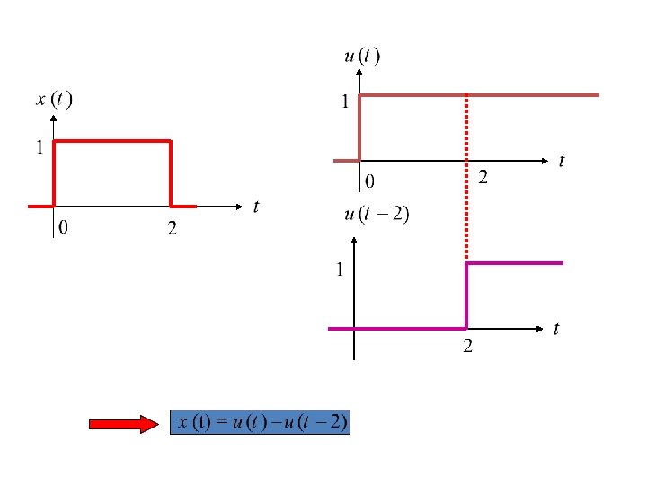
Pulse Function
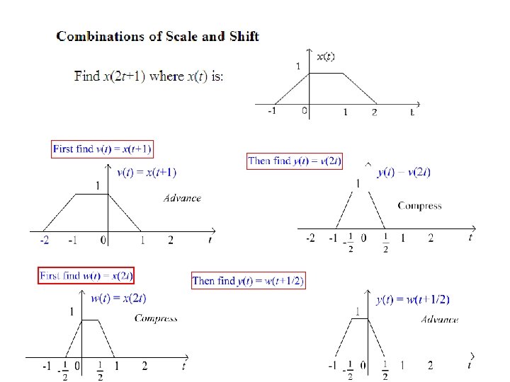
Chang of Scale Consider the pulse function P(t)
In general
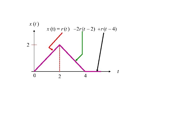
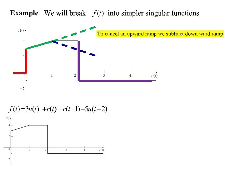
We want to express or decompose this function to singularities functions First we cancel the uprising ramp after t =2 with subtracting downward ramp Which will result in horizontal line segment However what we need is a downward ramp Therefore we need to subtract another ramp
However the downward ramp will continue indefinitely Therefore we need to cancel this part of downward ramp To cancel this part of downward ramp We add an upward ramp at t = 4
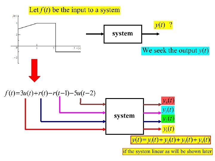
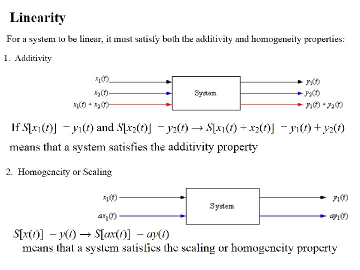
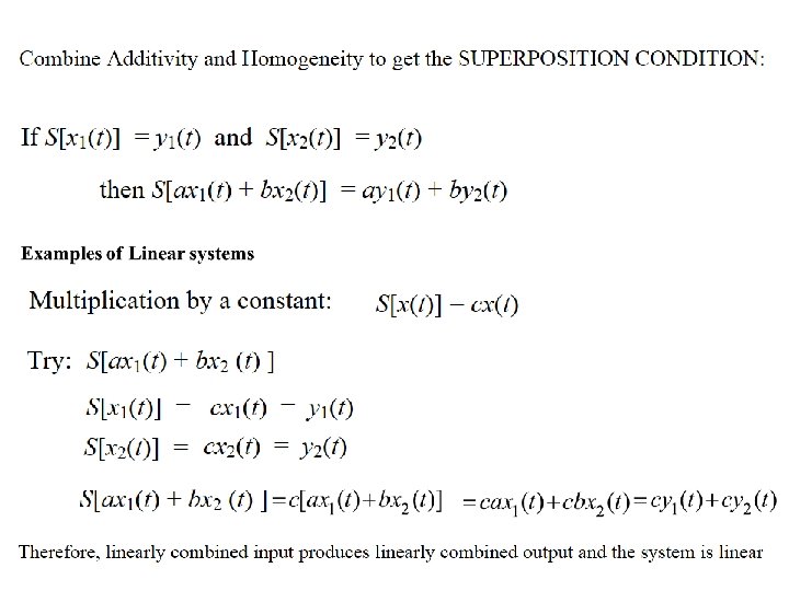
Input Output The relations between cause and effect (Input/output) are expressed as equations
Output Input Examples Electric Heater Car Speed paddle Speed
A another example of a physical system is a voltage amplifier such as that used in public-address systems amplifier block diagram
Representation of a general system y(t) = T[x(t)] where the notation T[x(t)] indicates a transformation or mapping This notation T[. ] does not indicate a function that is, T[x(t)] is not a mathematical function into which we substitute x(t) and directly calculate y(t). The explicit set of equations relating the input x(t) and the output y(t) is called the mathematical model, or simply, the model, of the system