TRANSFER LINES SPECIAL TOPICS Wolfgang Bartmann CAS Erice

TRANSFER LINES – SPECIAL TOPICS Wolfgang Bartmann CAS, Erice, March 2017

Outline • Introduction • What is a transfer line? • Paper studies 1 st hour • Geometry – estimate of bend angles • Optics – estimate of quadrupole gradients and apertures • Error estimates and tolerances on fields • Examples of using MADX for • • Optics and survey matching Achromats Final focus matching Error and correction studies 2 nd hour • Special cases in transfer lines • • • Particle tracking Stray fields Plane exchange Tilt on a slope Dilution 3 rd hour

Particle tracking • Numerical integration through field maps – ELENA beam lines • Tail population due to damped injection error – SPS ion injection • Scattering in collimators • Special processes like slow extraction – see Phil Bryant’s lecture

Tracking through field maps • Certain magnetic elements might not be ‘built-in’ elements in our code • Can use simulated/measured field maps and track particles through • ELENA transfer lines with 100 ke. V antiprotons • Transport via electrostatic elements • Quadrupole fields can be scaled wrt magnetic ones • Strong bends of up to 80 deg deflection require treatment as field maps

ELENA beam lines optics • First order optics established with MADX • Field maps simulated in COMSOL • Particles tracked through field maps in TRACK • Numerical integration of 6 D equation of motion through any type of field map • Track evaluates the Twiss parameters from a statistical distribution • Difference due to quadrupole hard-edge approximation in MADX – most visible in final focus where gradients are strongest M. Fraser

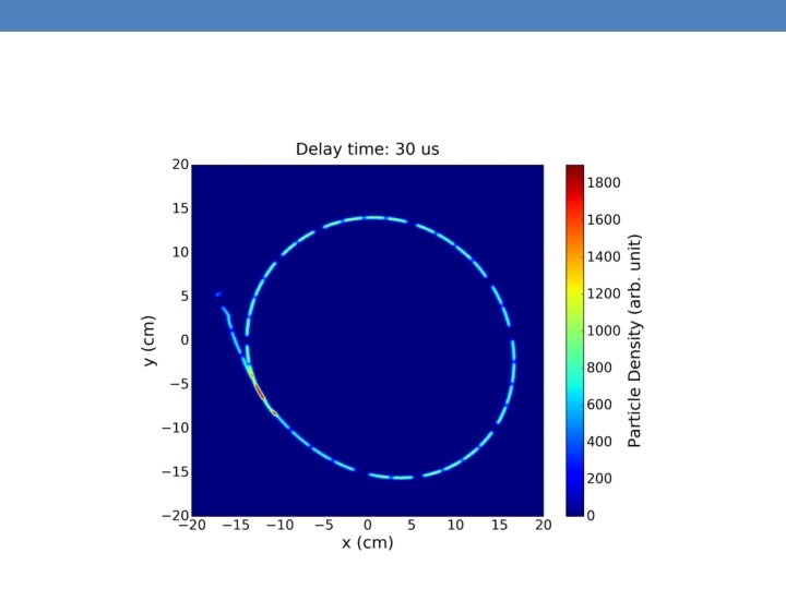
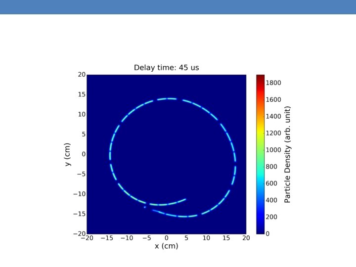
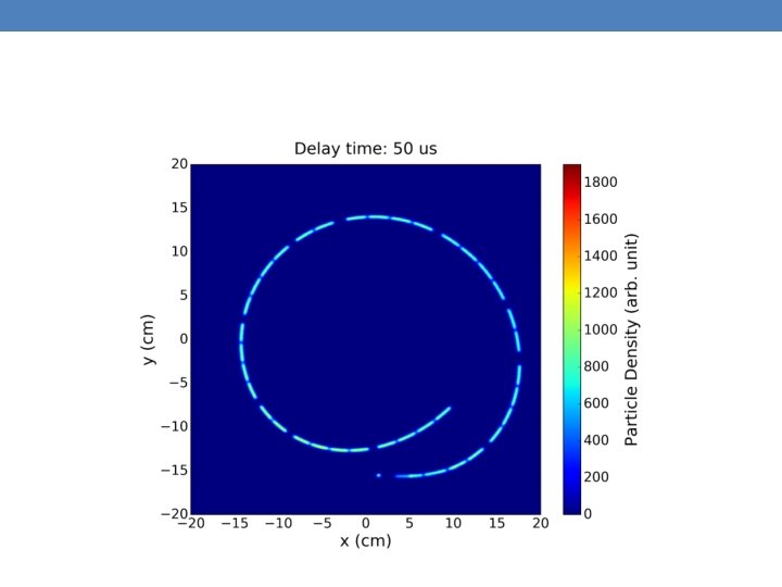
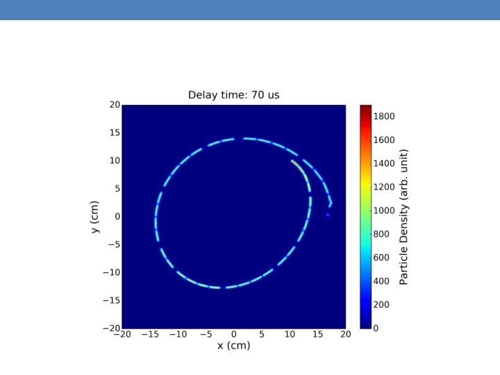
Particle tracking – Tail population at injection • LHC ion program profits a lot from reduced batch spacing at SPS injection • First and last bunches of a batch suffer from injection kick error – to a big part mitigated by the transverse damper • No effect on within measurement precision but increased population of tails observed from losses on transfer line collimators • How to simulate this? • Describe motion through accelerator by effective Hamiltonian formalism • Using Lie algebra to establish a One Turn Map • At turn 0 particles get an injection error, in later turns they see a damping effect from the transverse feedback Francesco Velotti

Particle tracking • Need to measure amplitude dependent detuning to define the coefficients of the effective Hamiltonian • Chromatic terms and damper gain estimated from decoherence measurements

Particle tracking Evaluate particle displacement after several thousands of turns

ELENA strayfields • Experimental solenoids of 1 -5 T magnetic field close to 100 ke. V beam line • How to simulate the impact on the beam? • Model the solenoids’ magnetic field with analytic description of current loops • Translate integrated transversal field components along beam line into horizontal and vertical kicks J. Mertens

ELENA strayfields • Effect of strayfield kicks on trajectory • Correction is required to stay within aperture • Problem: the strayfields depend on the state of the experimental magnets and no feedforward correction can be applied

Stray field attenuation • For a stray field attenuation of a factor 50, the trajectories can be corrected to 1 e-5 level • An attenuation of factor 800 is needed if different experimental magnet states have an effect on the trajectory at the same level as expected shot-to-shot variations

PS injection strayfield Magnetic field at transfer line was measured and translated into multipole kicks every 2 cm along the last meters before injection

Outline • Introduction • What is a transfer line? • Paper studies 1 st hour • Geometry – estimate of bend angles • Optics – estimate of quadrupole gradients and apertures • Error estimates and tolerances on fields • Examples of using MADX for • • Optics and survey matching Achromats Final focus matching Error and correction studies 2 nd hour • Special cases in transfer lines • • • Particle tracking Stray fields Plane exchange Tilt on a slope Dilution 3 rd hour

Emittance exchange insertion • Acceptances of circular accelerators tend to be larger in horizontal plane (bending dipole gap height small as possible) • Several multiturn extraction process produce beams which have emittances which are larger in the vertical plane larger losses • We can overcome this by exchanging the H and V phase planes (emittance exchange) Low energy machine y x After multi-turn extraction After emittance exchange High energy machine

Emittance exchange Phase-plane exchange requires a transformation of the form: A skew quadrupole is a normal quadrupole rotated by 45 deg. The transfer matrix S obtained by a rotation of the normal transfer matrix Mq: S = R-1 Mq. R where R is the rotation matrix (you can convince yourself of what R does by checking that x 0 is transformed to x 1 = x 0 cosq +y 0 sinq, y 0 into -x 0 sinq +y 0 cosq, etc. )

Emittance exchange For a thin-lens approximation (where d = kl = 1/f is the quadrupole strength) So that 45º skew quad For the case of q = 45º, this reduces to Normal quad

Emittance exchange The transformation required can be achieved with 3 such skew quads in a lattice, of strengths d 1, d 2, d 3, with transfer matrices S 1, S 2, S 3 A B Skew quad d 1 Skew quad d 2 d 3 The transfer matrix without the skew quads is C = B A. and similar for Cy

Emittance exchange With the skew quads the overall matrix is M = S 3 B S 2 A S 1 Equating the terms with our target matrix form a list of conditions result which must be met for phase-plane exchange.

Emittance exchange The simplest conditions are c 12 = c 34 = 0. Looking back at the matrix C, this means that Dfx and Dfy need to be integer multiples of p (i. e. the phase advance from first to last skew quad should be 180º, 360º, …) We also have for the strength of the skew quads

Emittance exchange Several solutions exist which give M the target form. One of the simplest is obtained by setting all the skew quadrupole strengths the same, and putting the skew quads at symmetric locations in a 90º FODO lattice A d B (=A) d d From symmetry A = B, and the values of a and b at all skew quads are identical. Therefore The matrix C is similar, but with phase advances of 2 Df with the same form for y

Emittance exchange Since we have chosen a 90º FODO phase advance, Dfx = Dfy = p/2, and 2 Dfx = 2 Dfy = p which means we can now write down A, B and C: i. e. 180º across the insertion in both planes we can then write down the skew lens strength as For the 90º FODO with half-cell length L,

If you got lost in the last 8 slides… …skew quadrupoles can tilt beams around their longitudinal axis Can there be any other (well known) beam line element do the same?

Beam tilt from dipoles …skew quadrupoles can tilt beams around their longitudinal axis. Can there be any other (well known) beam line element do the same? A horizontal dipole aligned on a slope introduces a tilt of the beam: Bend angle Slope angle

Beam tilt from dipoles • Effect from a single dipole small and in the order of misalignment • Becomes significant when accumulated over many dipoles along a transfer line • This gives 65 mrad roll angle for TI 8 • LHC itself is inclined but usually we calculate rings as if they were located in x-z plane and survey becomes 2 D, tilt and roll angle are 0 • If you consider the inclination of LHC you see that the tilt and roll angle oscillate but are perfectly closed after one turn B. Goddard

Beam tilt from dipoles • LHC has local tilt of 13 mrad at the injection point • Beam will be mismatched emittance growth • In case of LHC has negligible effect of ~1% • Trajectories must be matched, ideally in all 6 geometric degrees of freedom (x, y, z, theta, phi, psi) • MADX is correctly taking into account the roll angle calculation for dipoles on a slope • We just have to remember to calculate the local value of psi for a ring at the injection point

Outline • Introduction • What is a transfer line? • Paper studies 1 st hour • Geometry – estimate of bend angles • Optics – estimate of quadrupole gradients and apertures • Error estimates and tolerances on fields • Examples of using MADX for • • Optics and survey matching Achromats Final focus matching Error and correction studies 2 nd hour • Special cases in transfer lines • • • Particle tracking Stray fields Plane exchange Tilt on a slope Dilution 3 rd hour

Dilution Why do we need dilution?

Hydrodynamic tunneling test • Bunch spacing: 50 ns • Bunch trains with 36 bunches • Bunch intensity: 1. 5 E 11 p Florian Burkart

Back

Without dilution: • LHC beam would drill ~35 m hole into copper • For FCC ~300 m in copper Back

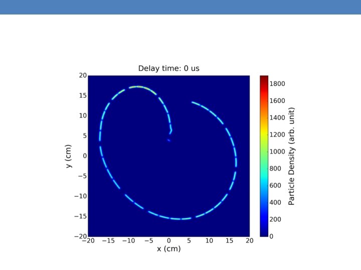
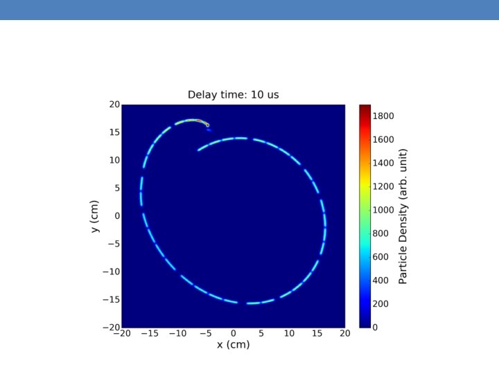
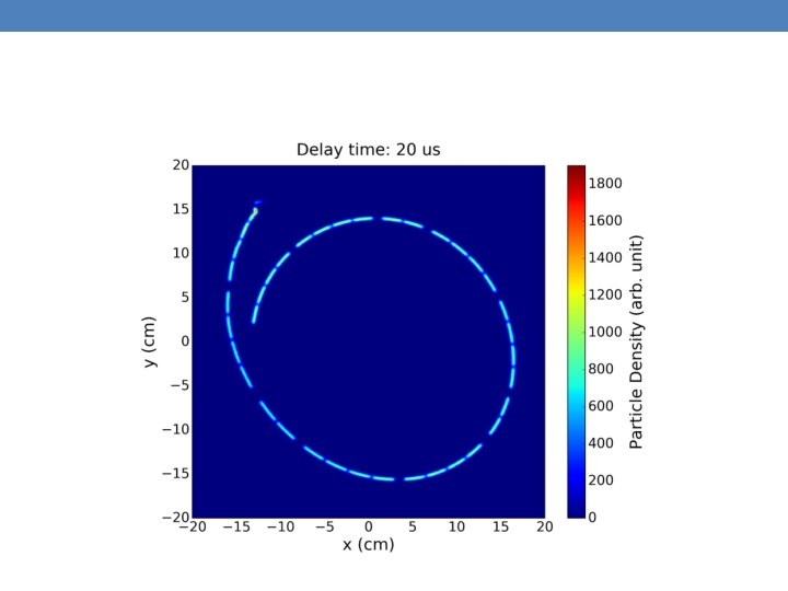
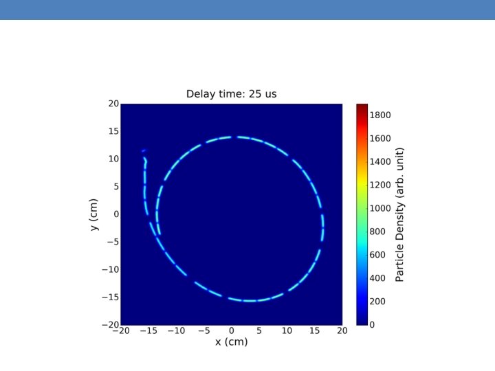
Dilution pattern • Could use inverse of final focus but in case of LHC, FCC this would lead to enormous absorber dimensions • Use time-varying dipole fields instead • Each bunch of the machine sees a slightly different deflection • Particle density on the dump block • From this pattern one has to study the shower development inside the block to define damage limits – see Anton Lechner’s lecture

Kicker erratics • Different approaches to handle the erratic: • Fire all the remaining as soon as you detect the erratic of one – LHC philosophy • Unsynchronised with the beam – will spray particles around the aperture which requires passive protection elements • Dump channel aperture is designed to accept also a beam deflected by one kicker less (14/15) • Ignore a single switch erratic – being studied for FCC • The effect of a single kicker on the beam should then be small ~ 1 sigma • Wait until the abort gap is in sync with the kicker and deflect the beam in a clean way into the dump channel • With 8 GJ circulating you want to make sure that the collimation system is fine with that • Also, one beam is kicked, but the other one will see a ‘coupling’ via beam-beam effects

LHC situation • Firing all the others in case of single failure is only done for the LHC extraction kickers – not for the dilution kickers • Also the dilution kickers switches are prone to fire spontaneously (a few per year) • Problem: EM coupling

LHC situation Spontaneous trigger time delay between MKBs For t ∞ αmax 75% (loss of 1 MKBH) For t ∞ αmax 50% (loss of 2 MKBH) For t ∞ αmax 25% (loss of 3 MKBH) For t ∞ αmax 0% (loss of 4 MKBH) 3/9/2021 MKB Retriggering C. Wiesner 34

LHC situation • Firing all the others in case of single failure is only done for the LHC extraction kickers – not for the dilution • We know since longer that also the dilution kickers switches are prone to fire spontaneously (a few per year) • Problem: EM coupling • Solution could be to retrigger them all – preferably in sync with the abort gap of the beam • This means that the time between the extraction kickers firing and the dilution kickers firing is not anymore constant • The dilution pattern on the dump will change

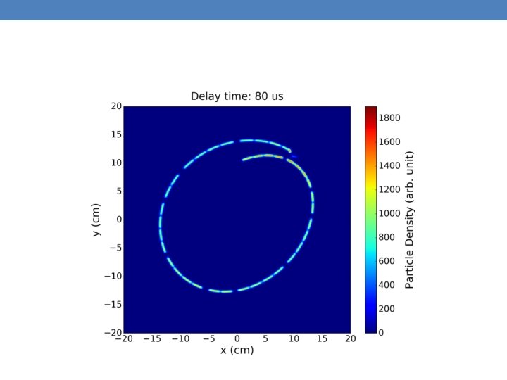
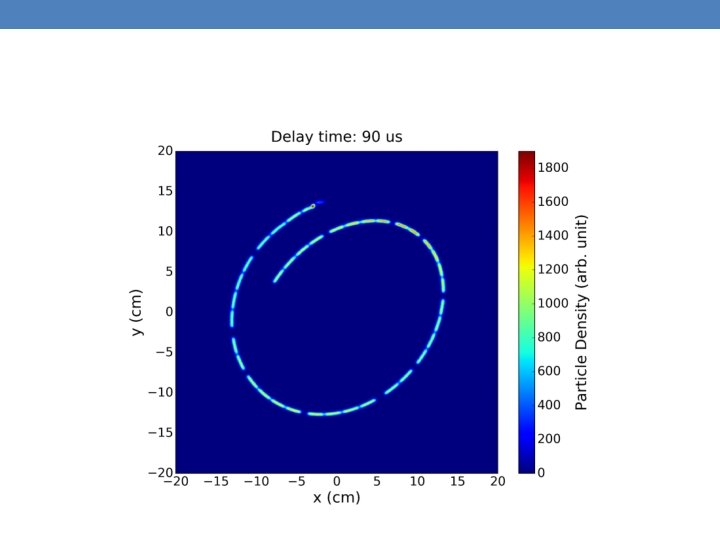
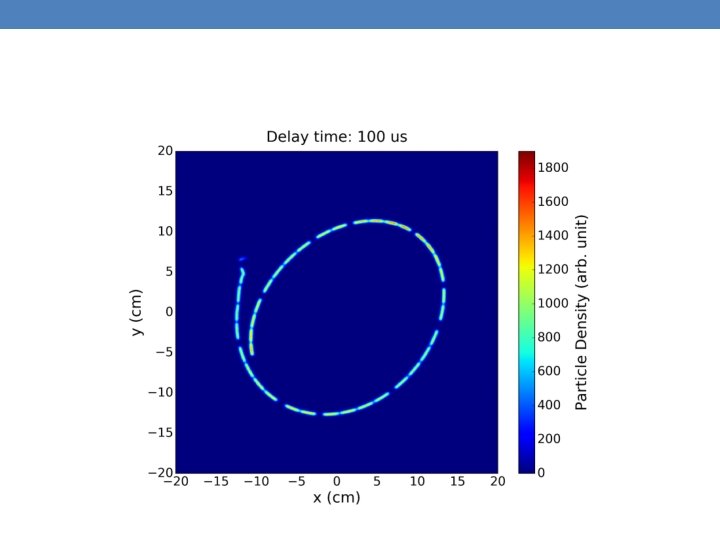
Particle density on dump face

Longitudinal peak dose profile • Particle density on dump face is not the full picture – see Anton’s lecture

Studies for FCC dilution pattern

Combine dilution with optics D. Barna • Horizontal kick enhanced by quadrupole kick due to off-centre passage • Vertical kickers aperture reduced in the critical plane • Looks like a good application of point-to-point focusing technique • Or using doublets with • point-to-parallel focusing • some equipment like instrumentation and vacuum • parallel to point focusing

Design of a dump system requires • Detailed knowledge of kicker hardware (see Mike’s lecture) • Waveforms, failure cases, coupling between systems • Simulations of particle-matter interactions (see Anton’s lecture) • Shower development • Knowledge of beam optics • Focusing system can reduce the dilution hardware requirements • Overall machine protection aspects of the ring • Can we afford to ignore a single kicker erratic (collimation, beam-beam, …)?

Summary for all TL lectures • Before switching on a computer we can define for a transfer line • Number of dipoles and quadrupoles, correctors and monitors • Dipole field and quadrupole tip field • Aperture of magnets and beam instrumentation • Rough estimate of required field quality and alignment accuracy • With computer codes • We can calculate the optics for matching sections and final focus for fixed target beams • Give a precise value for the field in each dipole and quadrupole • We can run error and correction studies • Define misalignment tolerances • Define field homogeneity and ripple • Define specifications for transverse feedback systems • Define sensitivity of instrumentation

Summary for all TL lectures • Certain cases require particle tracking • Numerically through field maps – for special elements which are not ‘built-in’ • Establishing the Hamiltonian and tracking particles with one turn maps – tail population after injection error • Particle distribution trough collimators – particle-matter interaction • Lines on the energy extremities provide special challenges • Stray-field calculation, measurement and shielding – 100 ke. V ELENA transfer lines next to 5 T solenoids • Dilution of high energy beams – LHC, FCC

Thank you for your attention And many thanks to my colleagues for helpful input: R. Baartman, D. Barna, M. Barnes, C. Bracco, P. Bryant, F. Burkart, V. Forte, M. Fraser, B. Goddard, C. Hessler, D. Johnson, V. Kain, T. Kramer, A. Lechner, J. Mertens, R. Ostojic, J. Schmidt, L. Stoel, C. Wiesner