Transcriptome Analysis Song Li Introduction to Transcriptome Analysis

Transcriptome Analysis Song Li

Introduction to Transcriptome Analysis • Goal of transcriptome analysis – Differentially expressed genes/small RNA – Clustering/network analysis – Identify novel transcripts (w/o reference genome) • Types of transcriptome analysis – RNA-seq – Small RNA-seq – Ribo-seq, PEAT-seq, Poly. A-seq – Normalized RNA-seq (for linc. RNA)

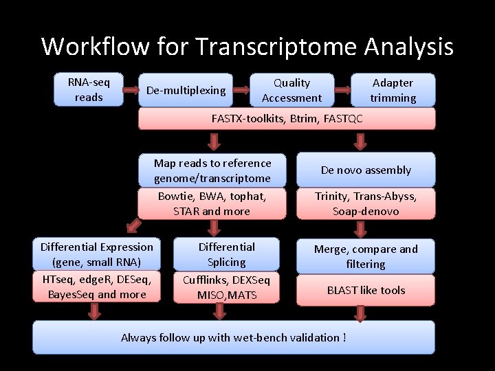
Workflow for Transcriptome Analysis RNA-seq reads De-multiplexing Quality Accessment Adapter trimming FASTX-toolkits, Btrim, FASTQC Map reads to reference genome/transcriptome Bowtie, BWA, tophat, STAR and more Differential Expression (gene, small RNA) HTseq, edge. R, DESeq, Bayes. Seq and more Differential Splicing Cufflinks, DEXSeq MISO, MATS De novo assembly Trinity, Trans-Abyss, Soap-denovo Merge, compare and filtering BLAST like tools Always follow up with wet-bench validation !

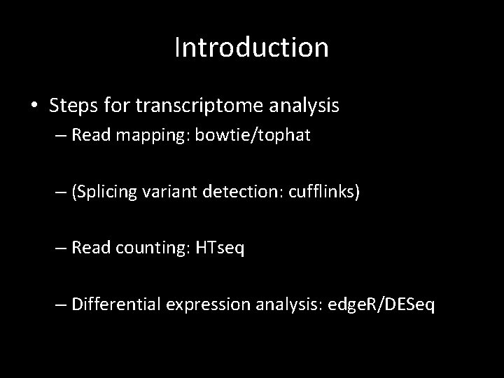
Introduction • Steps for transcriptome analysis – Read mapping: bowtie/tophat – (Splicing variant detection: cufflinks) – Read counting: HTseq – Differential expression analysis: edge. R/DESeq

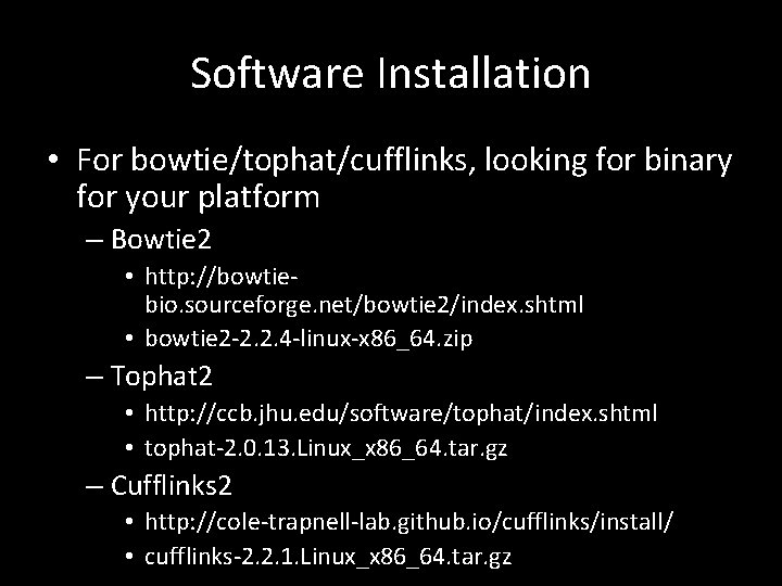
Software Installation • For bowtie/tophat/cufflinks, looking for binary for your platform – Bowtie 2 • http: //bowtiebio. sourceforge. net/bowtie 2/index. shtml • bowtie 2 -2. 2. 4 -linux-x 86_64. zip – Tophat 2 • http: //ccb. jhu. edu/software/tophat/index. shtml • tophat-2. 0. 13. Linux_x 86_64. tar. gz – Cufflinks 2 • http: //cole-trapnell-lab. github. io/cufflinks/install/ • cufflinks-2. 2. 1. Linux_x 86_64. tar. gz

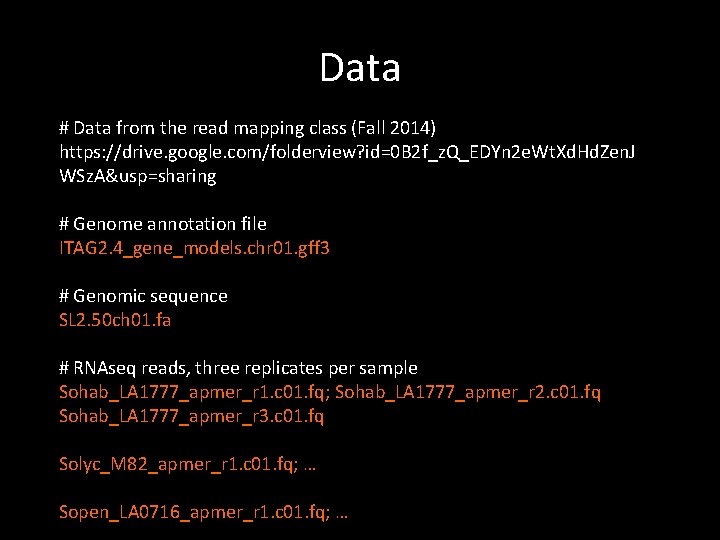
Data # Data from the read mapping class (Fall 2014) https: //drive. google. com/folderview? id=0 B 2 f_z. Q_EDYn 2 e. Wt. Xd. Hd. Zen. J WSz. A&usp=sharing # Genome annotation file ITAG 2. 4_gene_models. chr 01. gff 3 # Genomic sequence SL 2. 50 ch 01. fa # RNAseq reads, three replicates per sample Sohab_LA 1777_apmer_r 1. c 01. fq; Sohab_LA 1777_apmer_r 2. c 01. fq Sohab_LA 1777_apmer_r 3. c 01. fq Solyc_M 82_apmer_r 1. c 01. fq; … Sopen_LA 0716_apmer_r 1. c 01. fq; …

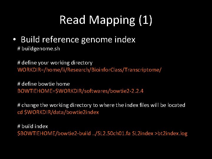
Read Mapping (1) • Build reference genome index # buildgenome. sh # define your working directory WORKDIR=/home/li/Research/Bioinfor. Class/Transcriptome/ # define bowtie home BOWTIEHOME=$WORKDIR/softwares/bowtie 2 -2. 2. 4 # change the working directory to where the index files will be located cd $WORKDIR/data/bowtie 2 index # build index $BOWTIEHOME/bowtie 2 -build. . /SL 2. 50 ch 01. fa SL 2 index >bt 2 index. log

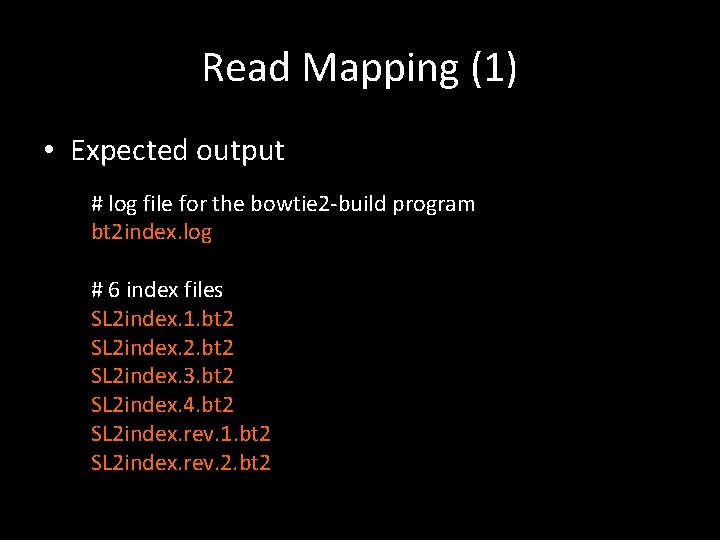
Read Mapping (1) • Expected output # log file for the bowtie 2 -build program bt 2 index. log # 6 index files SL 2 index. 1. bt 2 SL 2 index. 2. bt 2 SL 2 index. 3. bt 2 SL 2 index. 4. bt 2 SL 2 index. rev. 1. bt 2 SL 2 index. rev. 2. bt 2

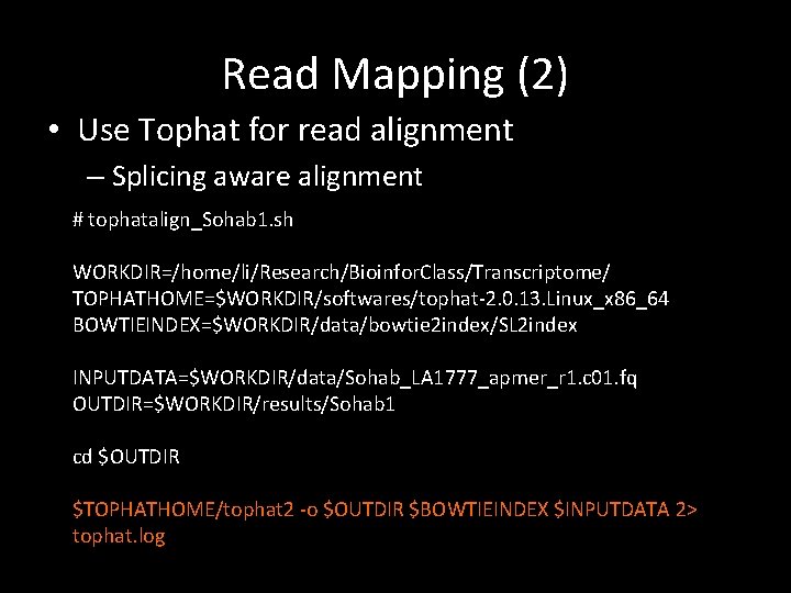
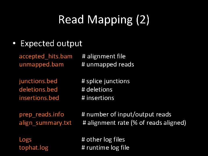
Read Mapping (2) • Use Tophat for read alignment – Splicing aware alignment # tophatalign_Sohab 1. sh WORKDIR=/home/li/Research/Bioinfor. Class/Transcriptome/ TOPHATHOME=$WORKDIR/softwares/tophat-2. 0. 13. Linux_x 86_64 BOWTIEINDEX=$WORKDIR/data/bowtie 2 index/SL 2 index INPUTDATA=$WORKDIR/data/Sohab_LA 1777_apmer_r 1. c 01. fq OUTDIR=$WORKDIR/results/Sohab 1 cd $OUTDIR $TOPHATHOME/tophat 2 -o $OUTDIR $BOWTIEINDEX $INPUTDATA 2> tophat. log

Read Mapping (2) • Expected output accepted_hits. bam unmapped. bam # alignment file # unmapped reads junctions. bed deletions. bed insertions. bed # splice junctions # deletions # insertions prep_reads. info align_summary. txt # number of input/output reads # alignment rate (% of reads aligned) Logs tophat. log # other log files # runtime log file

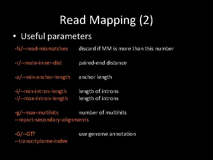
Read Mapping (2) • Useful parameters -N/--read-mismatches discard if MM is more than this number -r/--mate-inner-dist paired-end distance -a/--min-anchor-length anchor length -i/--min-intron-length -I/--max-intron-length of introns -g/--max-multihits number of multihits --report-secondary-alignments -G/--GTF --transcriptome-index use genome annotation

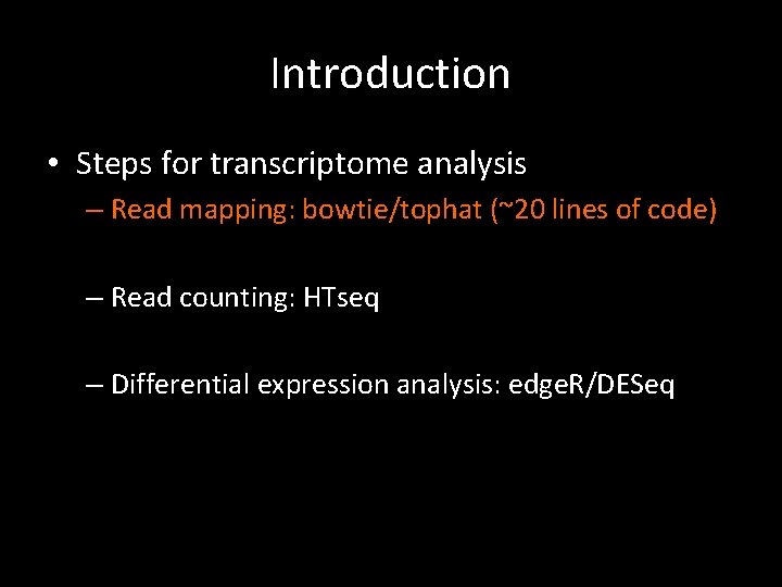
Introduction • Steps for transcriptome analysis – Read mapping: bowtie/tophat (~20 lines of code) – Read counting: HTseq – Differential expression analysis: edge. R/DESeq

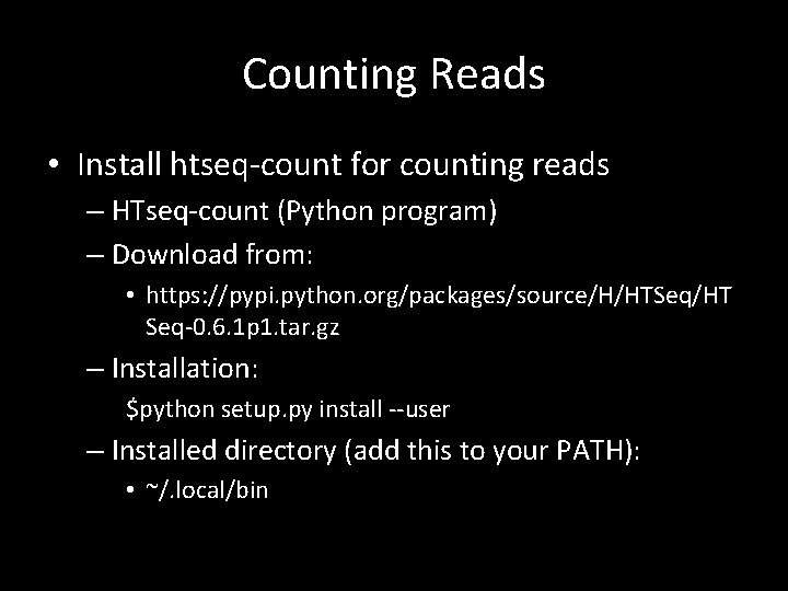
Counting Reads • Install htseq-count for counting reads – HTseq-count (Python program) – Download from: • https: //pypi. python. org/packages/source/H/HTSeq/HT Seq-0. 6. 1 p 1. tar. gz – Installation: $python setup. py install --user – Installed directory (add this to your PATH): • ~/. local/bin

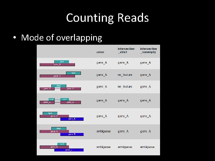
Counting Reads • Mode of overlapping

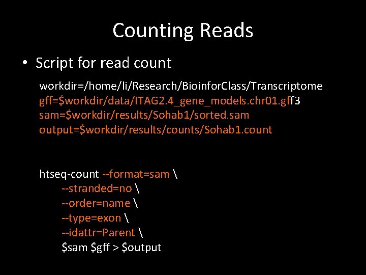
Counting Reads • Script for read count workdir=/home/li/Research/Bioinfor. Class/Transcriptome gff=$workdir/data/ITAG 2. 4_gene_models. chr 01. gff 3 sam=$workdir/results/Sohab 1/sorted. sam output=$workdir/results/counts/Sohab 1. count htseq-count --format=sam --stranded=no --order=name --type=exon --idattr=Parent $sam $gff > $output

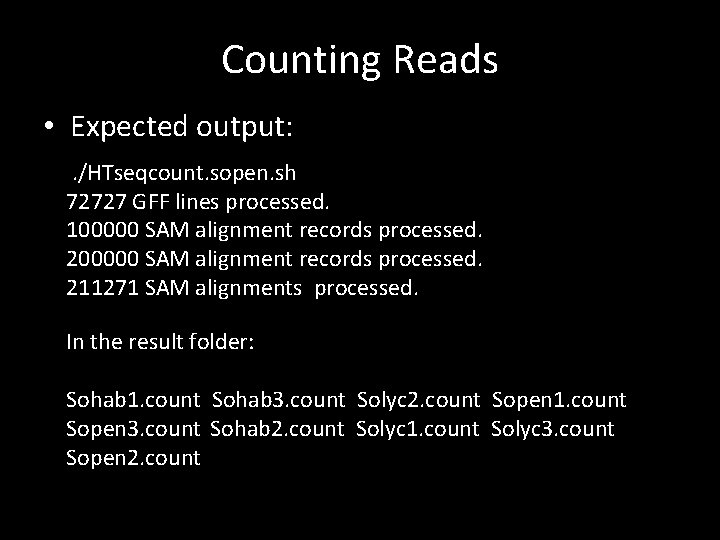
Counting Reads • Expected output: . /HTseqcount. sopen. sh 72727 GFF lines processed. 100000 SAM alignment records processed. 211271 SAM alignments processed. In the result folder: Sohab 1. count Sohab 3. count Solyc 2. count Sopen 1. count Sopen 3. count Sohab 2. count Solyc 1. count Solyc 3. count Sopen 2. count

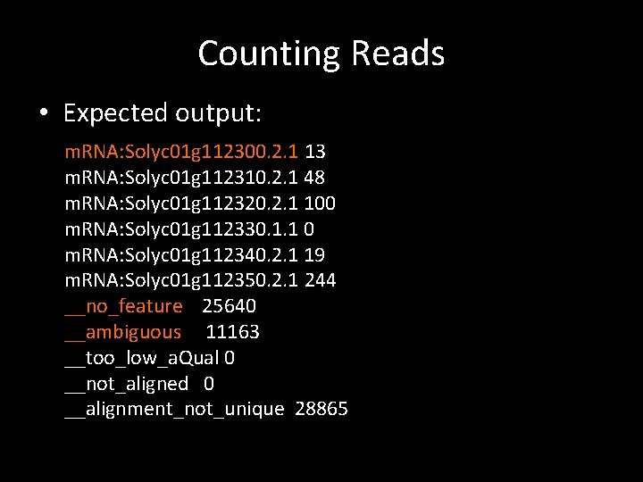
Counting Reads • Expected output: m. RNA: Solyc 01 g 112300. 2. 1 13 m. RNA: Solyc 01 g 112310. 2. 1 48 m. RNA: Solyc 01 g 112320. 2. 1 100 m. RNA: Solyc 01 g 112330. 1. 1 0 m. RNA: Solyc 01 g 112340. 2. 1 19 m. RNA: Solyc 01 g 112350. 2. 1 244 __no_feature 25640 __ambiguous 11163 __too_low_a. Qual 0 __not_aligned 0 __alignment_not_unique 28865

Introduction • Steps for transcriptome analysis – Read mapping: bowtie/tophat (~20 lines of code) – Read counting: Htseq (~10 lines of code) – Differential expression analysis: edge. R/DESeq

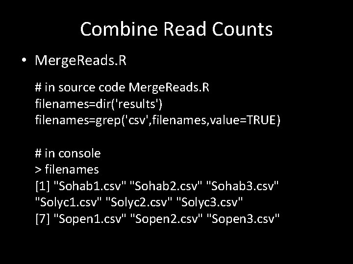
Combine Read Counts • Merge. Reads. R # in source code Merge. Reads. R filenames=dir('results') filenames=grep('csv', filenames, value=TRUE) # in console > filenames [1] "Sohab 1. csv" "Sohab 2. csv" "Sohab 3. csv" "Solyc 1. csv" "Solyc 2. csv" "Solyc 3. csv" [7] "Sopen 1. csv" "Sopen 2. csv" "Sopen 3. csv"

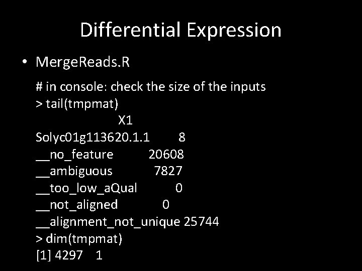
Differential Expression • Merge. Reads. R # in console: check the size of the inputs > tail(tmpmat) X 1 Solyc 01 g 113620. 1. 1 8 __no_feature 20608 __ambiguous 7827 __too_low_a. Qual 0 __not_aligned 0 __alignment_not_unique 25744 > dim(tmpmat) [1] 4297 1

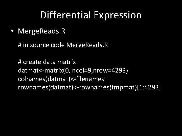
Differential Expression • Merge. Reads. R # in source code Merge. Reads. R # create data matrix datmat<-matrix(0, ncol=9, nrow=4293) colnames(datmat)<-filenames rownames(datmat)<-rownames(tmpmat)[1: 4293]

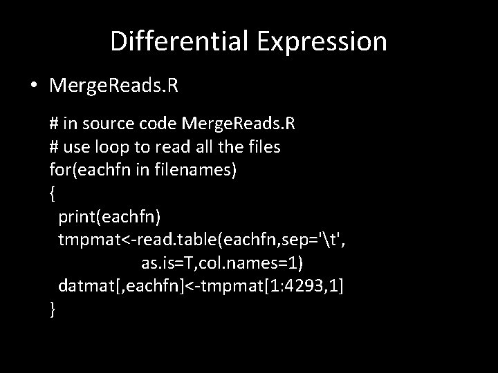
Differential Expression • Merge. Reads. R # in source code Merge. Reads. R # use loop to read all the files for(eachfn in filenames) { print(eachfn) tmpmat<-read. table(eachfn, sep='t', as. is=T, col. names=1) datmat[, eachfn]<-tmpmat[1: 4293, 1] }

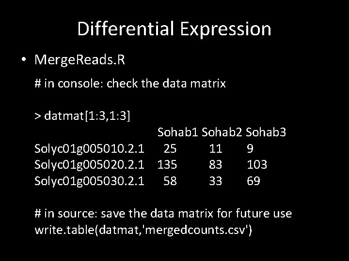
Differential Expression • Merge. Reads. R # in console: check the data matrix > datmat[1: 3, 1: 3] Sohab 1 Sohab 2 Sohab 3 Solyc 01 g 005010. 2. 1 25 11 9 Solyc 01 g 005020. 2. 1 135 83 103 Solyc 01 g 005030. 2. 1 58 33 69 # in source: save the data matrix for future use write. table(datmat, 'mergedcounts. csv')

Introduction • Steps for transcriptome analysis – Read mapping: bowtie/tophat (~20 lines of code) – Read counting: Htseq (< 10 lines of code) – Differential expression analysis: edge. R/DESeq • ~15 lines of code for data preparation

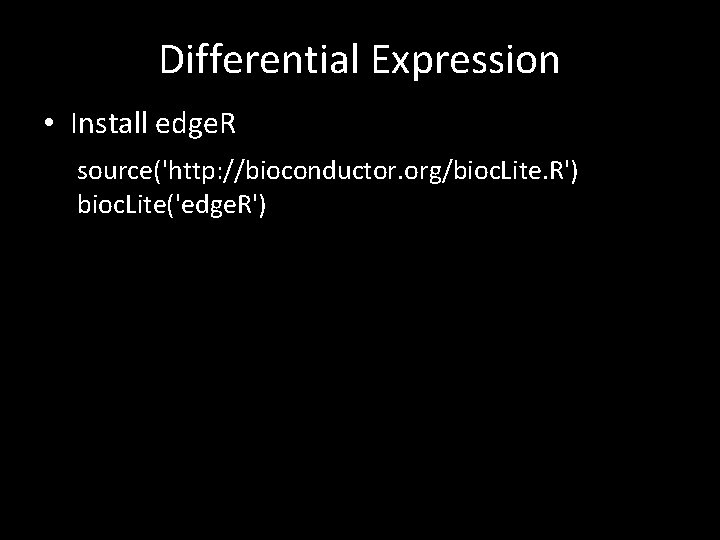
Differential Expression • Install edge. R source('http: //bioconductor. org/bioc. Lite. R') bioc. Lite('edge. R')

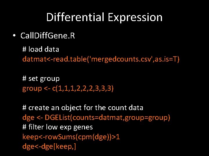
Differential Expression • Call. Diff. Gene. R # load data datmat<-read. table('mergedcounts. csv', as. is=T) # set group <- c(1, 1, 1, 2, 2, 2, 3, 3, 3) # create an object for the count data dge <- DGEList(counts=datmat, group=group) # filter low exp genes keep<-row. Sums(cpm(dge))>1 dge<-dge[keep, ]

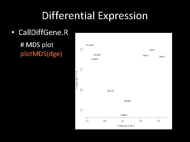
Differential Expression • Call. Diff. Gene. R # MDS plot. MDS(dge)

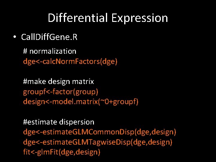
Differential Expression • Call. Diff. Gene. R # normalization dge<-calc. Norm. Factors(dge) #make design matrix groupf<-factor(group) design<-model. matrix(~0+groupf) #estimate dispersion dge<-estimate. GLMCommon. Disp(dge, design) dge<-estimate. GLMTagwise. Disp(dge, design) fit<-glm. Fit(dge, design)

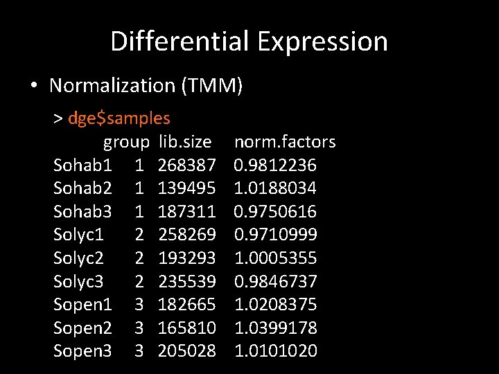
Differential Expression • Normalization (TMM) > dge$samples group lib. size Sohab 1 1 268387 Sohab 2 1 139495 Sohab 3 1 187311 Solyc 1 2 258269 Solyc 2 2 193293 Solyc 3 2 235539 Sopen 1 3 182665 Sopen 2 3 165810 Sopen 3 3 205028 norm. factors 0. 9812236 1. 0188034 0. 9750616 0. 9710999 1. 0005355 0. 9846737 1. 0208375 1. 0399178 1. 0101020

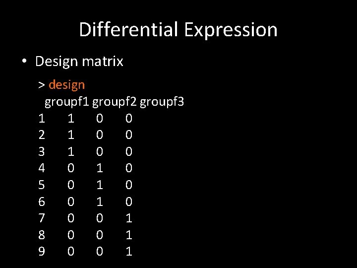
Differential Expression • Design matrix > design groupf 1 groupf 2 groupf 3 1 1 0 0 2 1 0 0 3 1 0 0 4 0 1 0 5 0 1 0 6 0 1 0 7 0 0 1 8 0 0 1 9 0 0 1

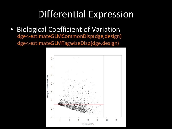
Differential Expression • Biological Coefficient of Variation dge<-estimate. GLMCommon. Disp(dge, design) dge<-estimate. GLMTagwise. Disp(dge, design)

Differential Expression • Call. Diff. Gene. R # normalization dge<-calc. Norm. Factors(dge) #make design matrix groupf<-factor(group) design<-model. matrix(~0+groupf) #estimate dispersion dge<-estimate. GLMCommon. Disp(dge, design) dge<-estimate. GLMTagwise. Disp(dge, design) fit<-glm. Fit(dge, design)

Differential Expression • Call. Diff. Gene. R # doing LRT test lrt. habvslyc<-glm. LRT(fit, contrast = c(1, -1, 0)) # select subset of genes tmpdiff<-top. Tags(lrt. habvslyc, n=1000) # filter by FDR diff. habvslyc<tmpdiff$table[, 5]<0. 05, ]

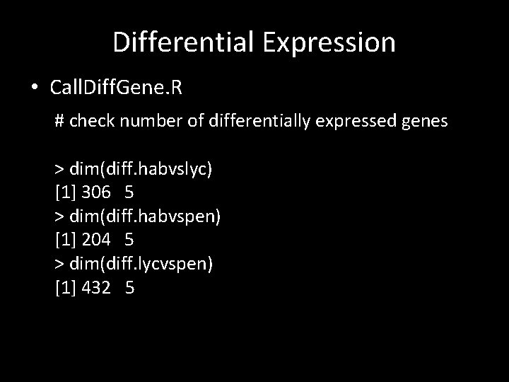
Differential Expression • Call. Diff. Gene. R # check number of differentially expressed genes > dim(diff. habvslyc) [1] 306 5 > dim(diff. habvspen) [1] 204 5 > dim(diff. lycvspen) [1] 432 5

Differential Expression • Call. Diff. Gene. R > diff. habvslyc[1: 2, ] log. FC log. CPM Solyc 01 g 106660. 1. 1 -3. 951948 8. 129906 Solyc 01 g 097520. 2. 1 3. 377053 11. 290468 LR PValue Solyc 01 g 106660. 1. 1 108. 63635 1. 949662 e-25 Solyc 01 g 097520. 2. 1 81. 23101 2. 008163 e-19 FDR Solyc 01 g 106660. 1. 1 8. 369899 e-22 Solyc 01 g 097520. 2. 1 4. 310522 e-16

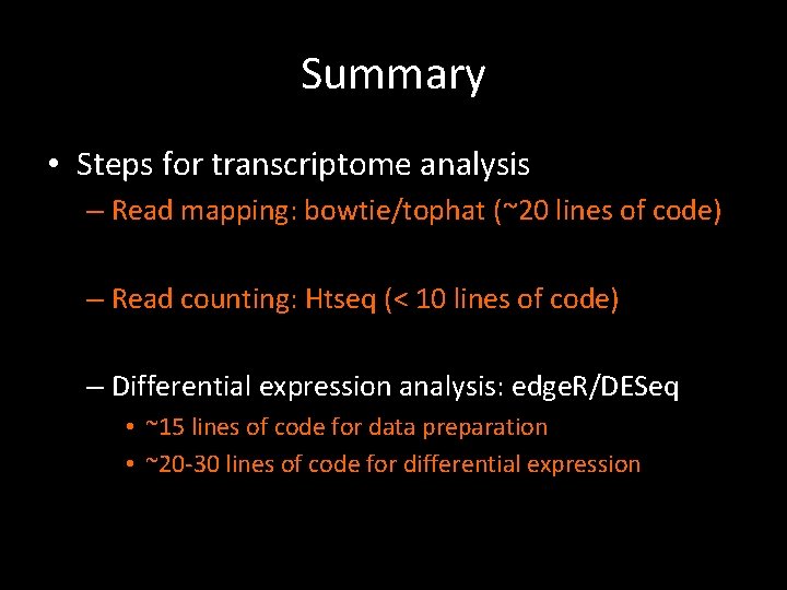
Summary • Steps for transcriptome analysis – Read mapping: bowtie/tophat (~20 lines of code) – Read counting: Htseq (< 10 lines of code) – Differential expression analysis: edge. R/DESeq • ~15 lines of code for data preparation • ~20 -30 lines of code for differential expression