Transcriptome Analysis Data Preprocessing Sample Preparation Illumina Sequencing

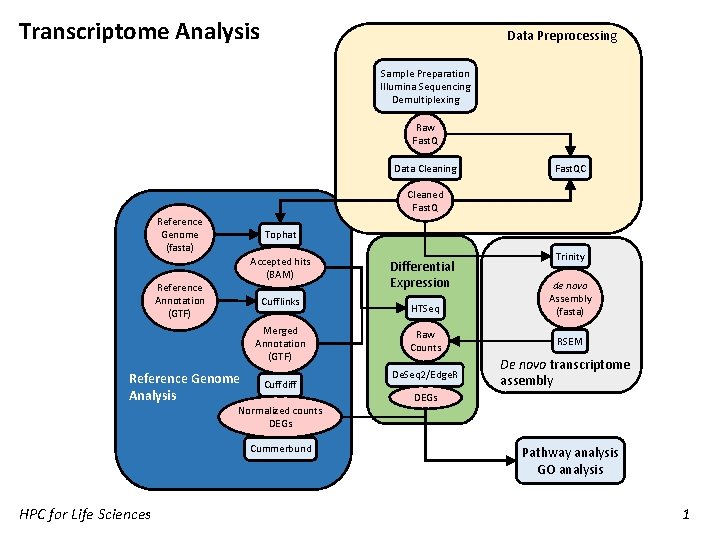
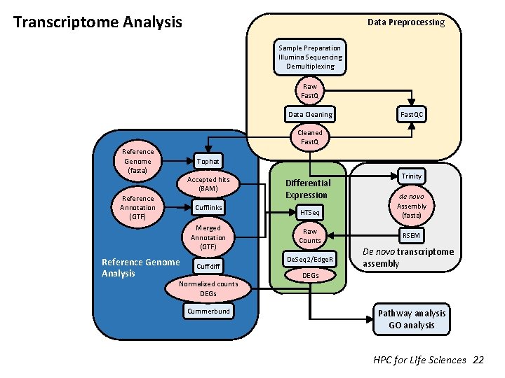
Transcriptome Analysis Data Preprocessing Sample Preparation Illumina Sequencing Demultiplexing Raw Fast. Q Data Cleaning Fast. QC Cleaned Fast. Q Reference Genome (fasta) Tophat Accepted hits (BAM) Reference Annotation (GTF) Cufflinks Merged Annotation (GTF) Reference Genome Analysis Cuffdiff Normalized counts DEGs Cummerbund HPC for Life Sciences Differential Expression HTSeq Raw Counts De. Seq 2/Edge. R Trinity de novo Assembly (fasta) RSEM De novo transcriptome assembly DEGs Pathway analysis GO analysis 1

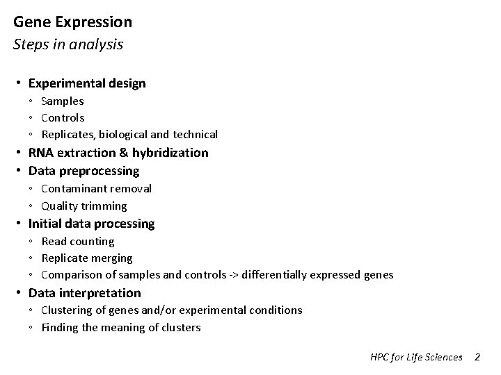
Gene Expression Steps in analysis • Experimental design ◦ Samples ◦ Controls ◦ Replicates, biological and technical • RNA extraction & hybridization • Data preprocessing ◦ Contaminant removal ◦ Quality trimming • Initial data processing ◦ Read counting ◦ Replicate merging ◦ Comparison of samples and controls -> differentially expressed genes • Data interpretation ◦ Clustering of genes and/or experimental conditions ◦ Finding the meaning of clusters HPC for Life Sciences 2

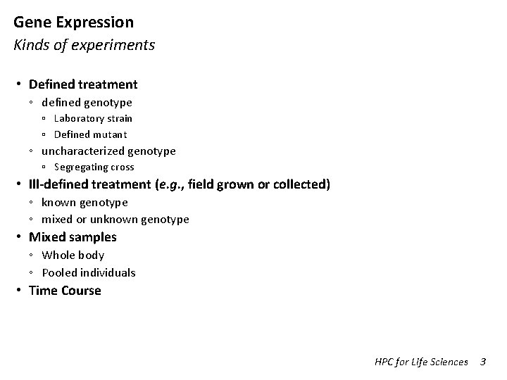
Gene Expression Kinds of experiments • Defined treatment ◦ defined genotype ▫ Laboratory strain ▫ Defined mutant ◦ uncharacterized genotype ▫ Segregating cross • Ill-defined treatment (e. g. , field grown or collected) ◦ known genotype ◦ mixed or unknown genotype • Mixed samples ◦ Whole body ◦ Pooled individuals • Time Course HPC for Life Sciences 3

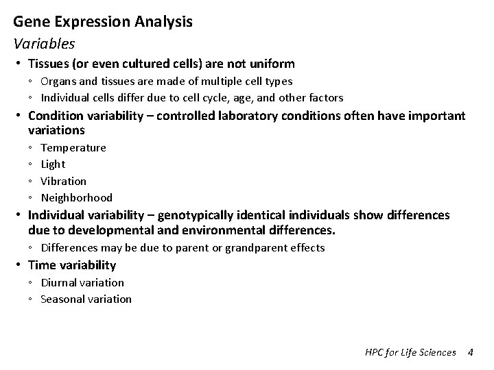
Gene Expression Analysis Variables • Tissues (or even cultured cells) are not uniform ◦ Organs and tissues are made of multiple cell types ◦ Individual cells differ due to cell cycle, age, and other factors • Condition variability – controlled laboratory conditions often have important variations ◦ ◦ Temperature Light Vibration Neighborhood • Individual variability – genotypically identical individuals show differences due to developmental and environmental differences. ◦ Differences may be due to parent or grandparent effects • Time variability ◦ Diurnal variation ◦ Seasonal variation HPC for Life Sciences 4

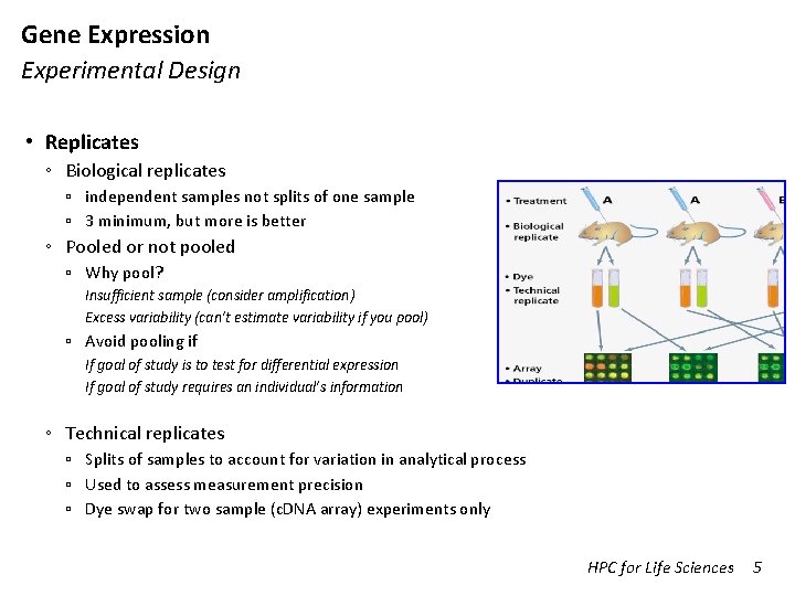
Gene Expression Experimental Design • Replicates ◦ Biological replicates ▫ independent samples not splits of one sample ▫ 3 minimum, but more is better ◦ Pooled or not pooled ▫ Why pool? Insufficient sample (consider amplification) Excess variability (can’t estimate variability if you pool) ▫ Avoid pooling if If goal of study is to test for differential expression If goal of study requires an individual’s information ◦ Technical replicates ▫ Splits of samples to account for variation in analytical process ▫ Used to assess measurement precision ▫ Dye swap for two sample (c. DNA array) experiments only HPC for Life Sciences 5

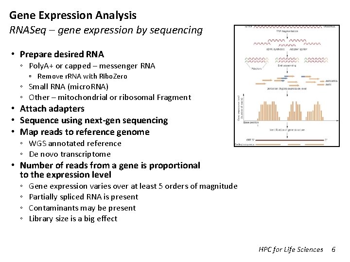
Gene Expression Analysis RNASeq – gene expression by sequencing • Prepare desired RNA ◦ Poly. A+ or capped – messenger RNA ▫ Remove r. RNA with Ribo. Zero ◦ Small RNA (micro. RNA) ◦ Other – mitochondrial or ribosomal Fragment • Attach adapters • Sequence using next-gen sequencing • Map reads to reference genome ◦ WGS annotated reference ◦ De novo transcriptome • Number of reads from a gene is proportional to the expression level ◦ ◦ Gene expression varies over at least 5 orders of magnitude Partially spliced RNA is present Contaminants may be present Library size is a big effect HPC for Life Sciences 6

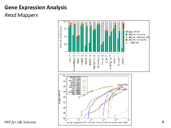
Gene Expression Analysis RNAseq • Next Generation sequencing technology ◦ 25 M – 1 G short reads (~100 - 150 bases) • Mapping to genome ◦ Blast type searches of 10 million queries against a genome can take days - too slow ◦ Fast mapping methods based on the Burrows-Wheeler transform are generally used: ▫ Bowtie 2, BWA, etc. ◦ Mapping methods may be splice-aware – better for RNA ▫ BBMap, HISAT, STAR, Subread, GSNAP, others HPC for Life Sciences 7

Gene Expression Analysis Read Mappers HPC for Life Sciences 8

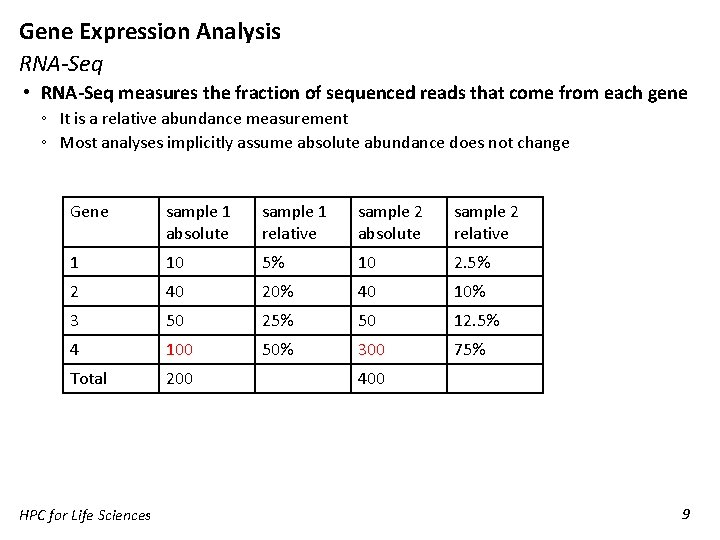
Gene Expression Analysis RNA-Seq • RNA-Seq measures the fraction of sequenced reads that come from each gene ◦ It is a relative abundance measurement ◦ Most analyses implicitly assume absolute abundance does not change Gene sample 1 absolute sample 1 relative sample 2 absolute sample 2 relative 1 10 5% 10 2. 5% 2 40 20% 40 10% 3 50 25% 50 12. 5% 4 100 50% 300 75% Total 200 HPC for Life Sciences 400 9

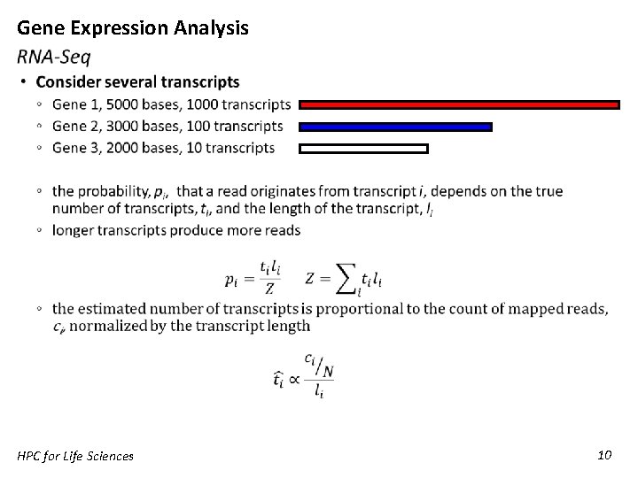
Gene Expression Analysis HPC for Life Sciences 10

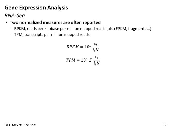
Gene Expression Analysis HPC for Life Sciences 11

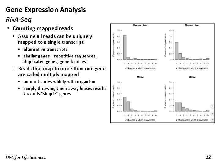
Gene Expression Analysis RNA-Seq • Counting mapped reads ◦ Assume all reads can be uniquely mapped to a single transcript ▫ alternative transcripts ▫ similar genes – repetitive sequences, duplicated genes, gene families ◦ Reads that map to more than one gene are called multiply mapped ▫ amount varies widely with organism ▫ simply throwing them away biases results towards “simple” genes HPC for Life Sciences 12

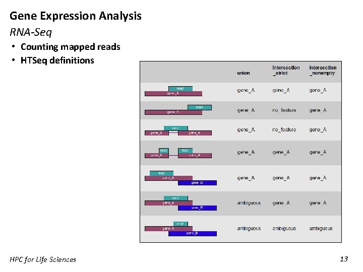
Gene Expression Analysis RNA-Seq • Counting mapped reads • HTSeq definitions HPC for Life Sciences 13

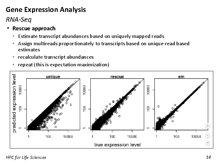
Gene Expression Analysis RNA-Seq • Rescue approach ◦ Estimate transcript abundances based on uniquely mapped reads ◦ Assign multireads proportionately to transcripts based on unique-read based estimates ◦ recalculate transcript abundances ◦ repeat (this is expectation maximization) HPC for Life Sciences 14

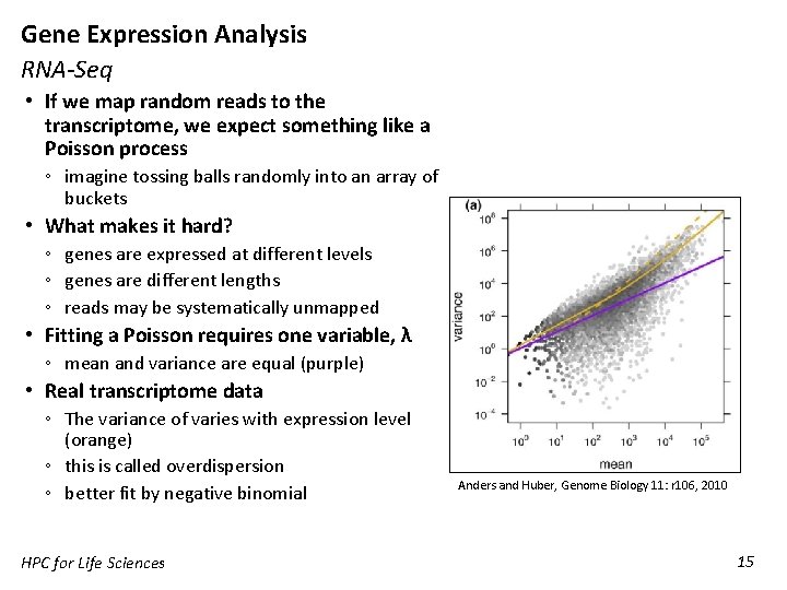
Gene Expression Analysis RNA-Seq • If we map random reads to the transcriptome, we expect something like a Poisson process ◦ imagine tossing balls randomly into an array of buckets • What makes it hard? ◦ genes are expressed at different levels ◦ genes are different lengths ◦ reads may be systematically unmapped • Fitting a Poisson requires one variable, λ ◦ mean and variance are equal (purple) • Real transcriptome data ◦ The variance of varies with expression level (orange) ◦ this is called overdispersion ◦ better fit by negative binomial HPC for Life Sciences Anders and Huber, Genome Biology 11: r 106, 2010 15

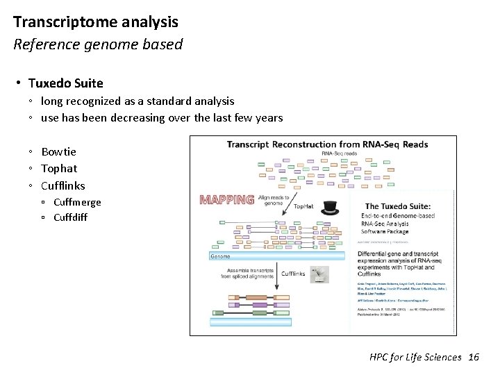
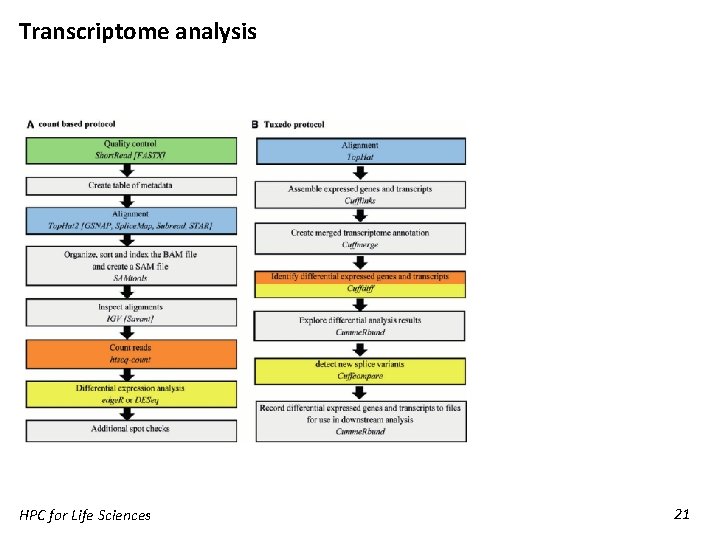
Transcriptome analysis Reference genome based • Tuxedo Suite ◦ long recognized as a standard analysis ◦ use has been decreasing over the last few years ◦ Bowtie ◦ Tophat ◦ Cufflinks ▫ Cuffmerge ▫ Cuffdiff HPC for Life Sciences 16

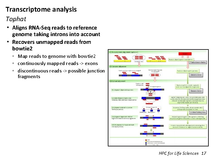
Transcriptome analysis Tophat • Aligns RNA-Seq reads to reference genome taking introns into account • Recovers unmapped reads from bowtie 2 ◦ Map reads to genome with bowtie 2 ◦ continuously mapped reads -> exons ◦ discontinuous reads -> possible junction fragments HPC for Life Sciences 17

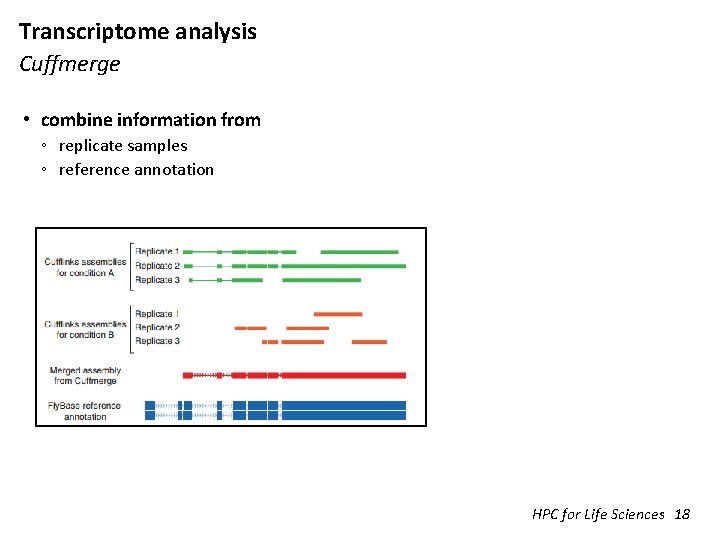
Transcriptome analysis Cuffmerge • combine information from ◦ replicate samples ◦ reference annotation HPC for Life Sciences 18

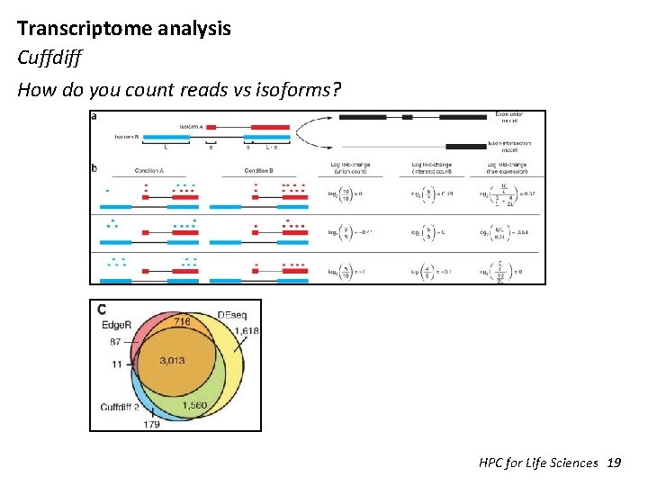
Transcriptome analysis Cuffdiff How do you count reads vs isoforms? HPC for Life Sciences 19

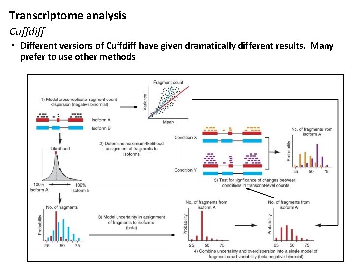
Transcriptome analysis Cuffdiff • Different versions of Cuffdiff have given dramatically different results. Many prefer to use other methods HPC for Life Sciences 20

Transcriptome analysis HPC for Life Sciences 21

Transcriptome Analysis Data Preprocessing Sample Preparation Illumina Sequencing Demultiplexing Raw Fast. Q Data Cleaning Fast. QC Cleaned Fast. Q Reference Genome (fasta) Tophat Accepted hits (BAM) Reference Annotation (GTF) Cufflinks Merged Annotation (GTF) Reference Genome Analysis Cuffdiff Normalized counts DEGs Cummerbund Differential Expression HTSeq Raw Counts De. Seq 2/Edge. R Trinity de novo Assembly (fasta) RSEM De novo transcriptome assembly DEGs Pathway analysis GO analysis HPC for Life Sciences 22

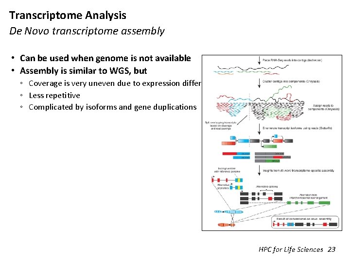
Transcriptome Analysis De Novo transcriptome assembly • Can be used when genome is not available • Assembly is similar to WGS, but ◦ Coverage is very uneven due to expression differences ◦ Less repetitive ◦ Complicated by isoforms and gene duplications HPC for Life Sciences 23

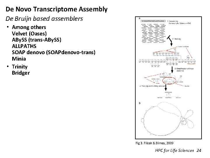
De Novo Transcriptome Assembly De Bruijn based assemblers • Among others Velvet (Oases) ABy. SS (trans-ABy. SS) ALLPATHS SOAP denovo (SOAPdenovo-trans) Minia • Trinity Bridger Fig 3. Flicek & Birney, 2009 HPC for Life Sciences 24

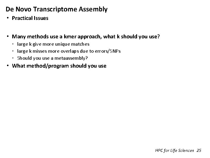
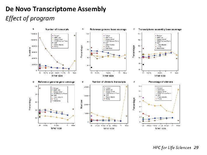
De Novo Transcriptome Assembly • Practical Issues • Many methods use a kmer approach, what k should you use? ◦ large k give more unique matches ◦ large k misses more overlaps due to errors/SNPs ◦ Should you use a metaassembly? • What method/program should you use HPC for Life Sciences 25

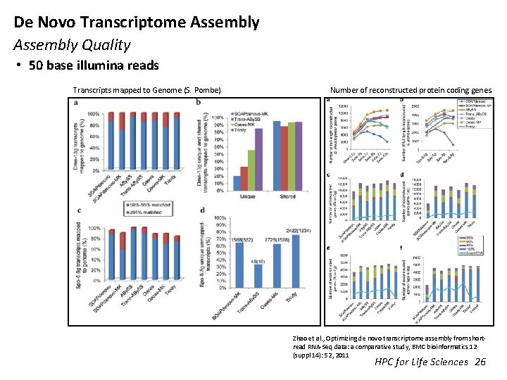
De Novo Transcriptome Assembly Quality • 50 base illumina reads Transcripts mapped to Genome (S. Pombe) Number of reconstructed protein coding genes. Zhao et al. , Optimizing de novo transcriptome assembly from shortread RNA-Seq data: a comparative study, BMC bioinformatics 12 (suppl 14): 52, 2011 HPC for Life Sciences 26

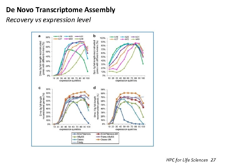
De Novo Transcriptome Assembly Recovery vs expression level HPC for Life Sciences 27

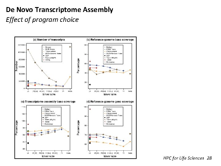
De Novo Transcriptome Assembly Effect of program choice HPC for Life Sciences 28

De Novo Transcriptome Assembly Effect of program HPC for Life Sciences 29

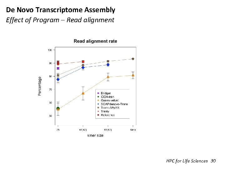
De Novo Transcriptome Assembly Effect of Program – Read alignment HPC for Life Sciences 30

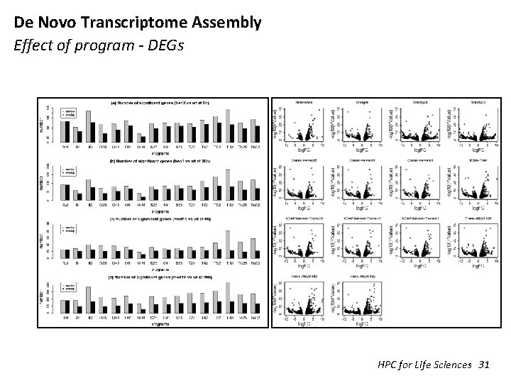
De Novo Transcriptome Assembly Effect of program - DEGs HPC for Life Sciences 31

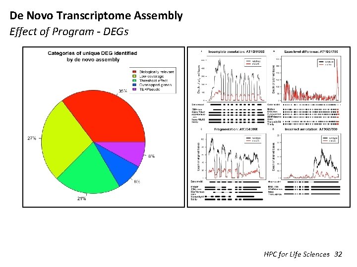
De Novo Transcriptome Assembly Effect of Program - DEGs HPC for Life Sciences 32

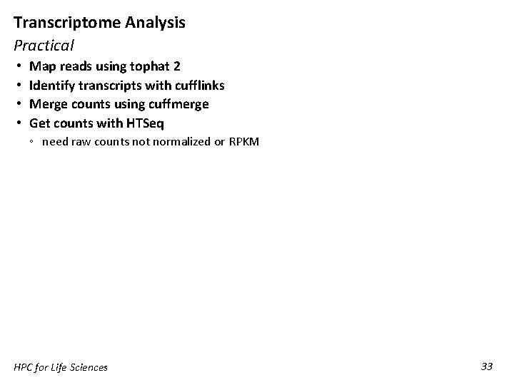
Transcriptome Analysis Practical • • Map reads using tophat 2 Identify transcripts with cufflinks Merge counts using cuffmerge Get counts with HTSeq ◦ need raw counts not normalized or RPKM HPC for Life Sciences 33

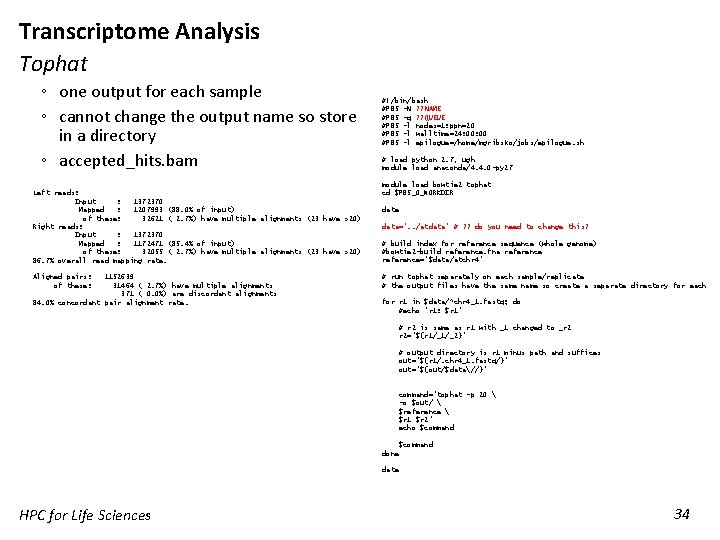
Transcriptome Analysis Tophat ◦ one output for each sample ◦ cannot change the output name so store in a directory ◦ accepted_hits. bam Left reads: Input : 1372370 Mapped : 1207993 (88. 0% of input) of these: 32621 ( 2. 7%) have multiple alignments (23 have >20) Right reads: Input : 1372370 Mapped : 1172471 (85. 4% of input) of these: 32055 ( 2. 7%) have multiple alignments (23 have >20) 86. 7% overall read mapping rate. Aligned pairs: of these: 1152639 31464 ( 2. 7%) have multiple alignments 371 ( 0. 0%) are discordant alignments 84. 0% concordant pair alignment rate. #!/bin/bash #PBS -N ? ? NAME #PBS -q ? ? QUEUE #PBS -l nodes=1: ppn=20 #PBS -l walltime=24: 00 #PBS -l epilogue=/home/mgribsko/jobs/epilogue. sh # load python 2. 7, ugh module load anaconda/4. 4. 0 -py 27 module load bowtie 2 tophat cd $PBS_O_WORKDIR date data=". . /atdata“ # ? ? do you need to change this? # build index for reference sequence (whole genome) #bowtie 2 -build reference. fna reference=“$data/atchr 4" # run tophat separately on each sample/replicate # the output files have the same name so create a separate directory for each for r 1 in $data/*chr 4_1. fastq; do #echo "r 1: $r 1" # r 2 is same as r 1 with _1 changed to _r 2 r 2="${r 1/_1/_2}" # output directory is r 1 minus path and suffices out="${r 1/. chr 4_1. fastq/}" out="${out/$data//}" command="tophat -p 20 -o $out/ $reference $r 1 $r 2" echo $command done date HPC for Life Sciences 34

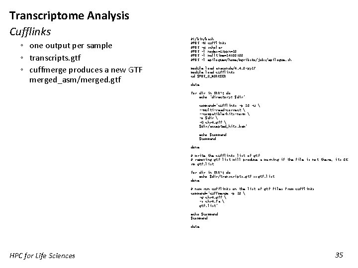
Transcriptome Analysis Cufflinks ◦ one output per sample ◦ transcripts. gtf ◦ cuffmerge produces a new GTF merged_asm/merged. gtf #!/bin/bash #PBS -N cufflinks #PBS -q scholar #PBS -l nodes=1: ppn=20 #PBS -l walltime=24: 00 #PBS -l epilogue=/home/mgribsko/jobs/epilogue. sh module load anaconda/4. 4. 0 -py 27 module load cufflinks cd $PBS_O_WORKDIR date for dir in SRR*; do echo "directory: $dir" command="cufflinks -p 20 -u --multi-read-correct --compatible-hits-norm -o $dir -G chr 4. gff $dir/accepted_hits. bam" echo $command done # write the cufflinks list of gtf # removing gtf list will produce a warning if the file is not there, its OK rm gtf. list for dir in SRR*; do echo $dir/transcripts. gtf >>gtf. list done # now run cufflinks on the list of gtf files from cufflinks command="cuffmerge -p 20 -g chr 4. gff -s chr 4. fa gtf. list" echo $command date HPC for Life Sciences 35

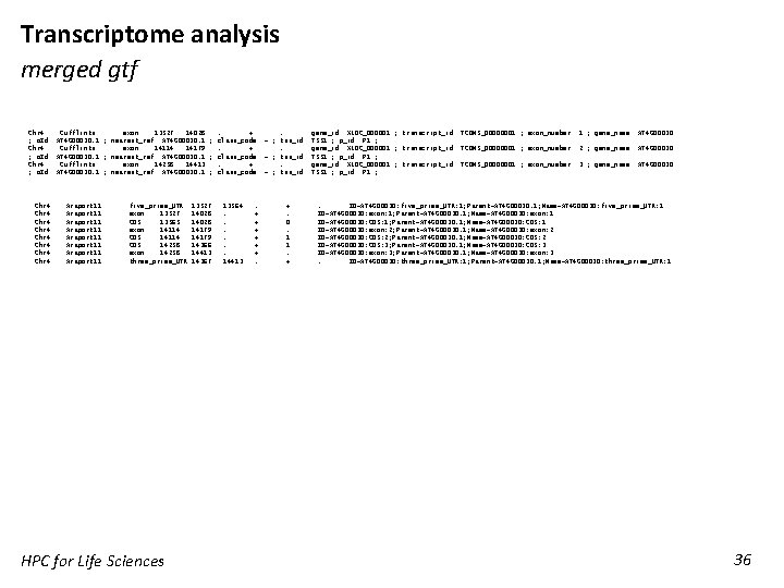
Transcriptome analysis merged gtf Chr 4 Cufflinks exon 13527 14028 ; o. Id "AT 4 G 00030. 1"; nearest_ref "AT 4 G 00030. 1"; Chr 4 Cufflinks exon 14114 14179 ; o. Id "AT 4 G 00030. 1"; nearest_ref "AT 4 G 00030. 1"; Chr 4 Cufflinks exon 14258 14413 ; o. Id "AT 4 G 00030. 1"; nearest_ref "AT 4 G 00030. 1"; Chr 4 Chr 4 Araport 11 Araport 11 five_prime_UTR exon 13527 CDS 13565 exon 14114 CDS 14258 exon 14258 three_prime_UTR HPC for Life Sciences 13527 14028 14179 14366 14413 14367 . +. gene_id "XLOC_000001"; transcript_id "TCONS_00000001"; exon_number "1"; gene_name "AT 4 G 00030" class_code "="; tss_id "TSS 1"; p_id "P 1"; . +. gene_id "XLOC_000001"; transcript_id "TCONS_00000001"; exon_number "2"; gene_name "AT 4 G 00030" class_code "="; tss_id "TSS 1"; p_id "P 1"; . +. gene_id "XLOC_000001"; transcript_id "TCONS_00000001"; exon_number "3"; gene_name "AT 4 G 00030" class_code "="; tss_id "TSS 1"; p_id "P 1"; 13564. . . 14413 . + + +. +. 0. 1 1. + . ID=AT 4 G 00030: five_prime_UTR: 1; Parent=AT 4 G 00030. 1; Name=AT 4 G 00030: five_prime_UTR: 1 ID=AT 4 G 00030: exon: 1; Parent=AT 4 G 00030. 1; Name=AT 4 G 00030: exon: 1 ID=AT 4 G 00030: CDS: 1; Parent=AT 4 G 00030. 1; Name=AT 4 G 00030: CDS: 1 ID=AT 4 G 00030: exon: 2; Parent=AT 4 G 00030. 1; Name=AT 4 G 00030: exon: 2 ID=AT 4 G 00030: CDS: 2; Parent=AT 4 G 00030. 1; Name=AT 4 G 00030: CDS: 2 ID=AT 4 G 00030: CDS: 3; Parent=AT 4 G 00030. 1; Name=AT 4 G 00030: CDS: 3 ID=AT 4 G 00030: exon: 3; Parent=AT 4 G 00030. 1; Name=AT 4 G 00030: exon: 3. ID=AT 4 G 00030: three_prime_UTR: 1; Parent=AT 4 G 00030. 1; Name=AT 4 G 00030: three_prime_UTR: 1 36

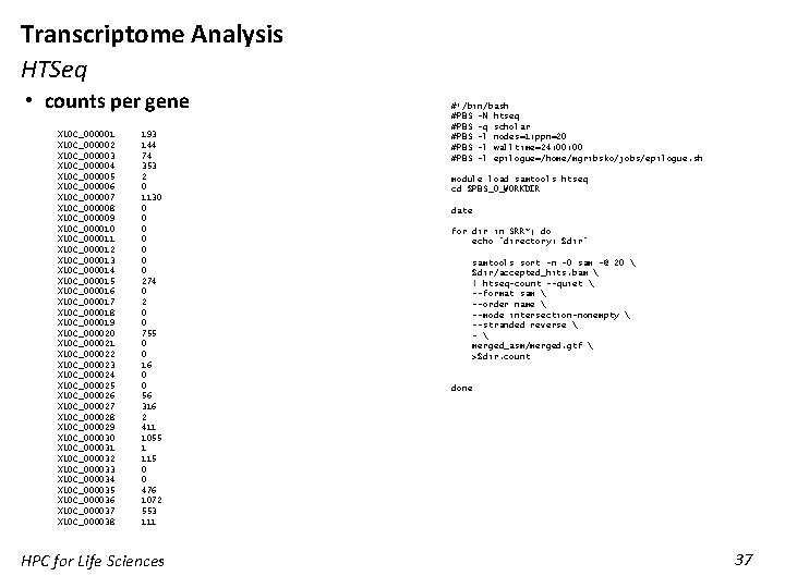
Transcriptome Analysis HTSeq • counts per gene XLOC_000001 XLOC_000002 XLOC_000003 XLOC_000004 XLOC_000005 XLOC_000006 XLOC_000007 XLOC_000008 XLOC_000009 XLOC_000010 XLOC_000011 XLOC_000012 XLOC_000013 XLOC_000014 XLOC_000015 XLOC_000016 XLOC_000017 XLOC_000018 XLOC_000019 XLOC_000020 XLOC_000021 XLOC_000022 XLOC_000023 XLOC_000024 XLOC_000025 XLOC_000026 XLOC_000027 XLOC_000028 XLOC_000029 XLOC_000030 XLOC_000031 XLOC_000032 XLOC_000033 XLOC_000034 XLOC_000035 XLOC_000036 XLOC_000037 XLOC_000038 193 144 74 353 2 0 1130 0 0 0 274 0 2 0 0 755 0 0 16 0 0 56 316 2 411 1055 1 115 0 0 476 1072 553 111 HPC for Life Sciences #!/bin/bash #PBS -N htseq #PBS -q scholar #PBS -l nodes=1: ppn=20 #PBS -l walltime=24: 00 #PBS -l epilogue=/home/mgribsko/jobs/epilogue. sh module load samtools htseq cd $PBS_O_WORKDIR date for dir in SRR*; do echo "directory: $dir" samtools sort -n -O sam -@ 20 $dir/accepted_hits. bam | htseq-count --quiet --format sam --order name --mode intersection-nonempty --stranded reverse - merged_asm/merged. gtf >$dir. count done 37

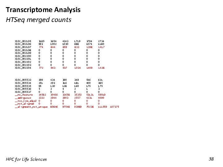
Transcriptome Analysis HTSeq merged counts XLOC_002195 XLOC_002196 XLOC_002197 XLOC_002198 XLOC_002199 XLOC_002200 XLOC_002201 XLOC_002202 XLOC_002203 XLOC_002204 3185 993 774 0 0 0 772 XLOC_005533 299 XLOC_005534 251 XLOC_005535 95 XLOC_005536 5 XLOC_005537 0 __no_feature 24582 __ambiguous 2332 __too_low_a. Qual 0 __not_aligned 0 __alignment_not_unique HPC for Life Sciences 3654 1002 844 0 0 0 963 4343 1030 859 0 0 0 937 1719 688 833 0 0 0 1034 3794 1074 1398 0 0 0 1409 2734 1180 1417 0 0 0 1428 434 293 130 2 0 30492 2944 0 0 80846 390 316 128 4 0 32658 2903 0 0 97548 349 181 160 2 0 35352 2557 0 0 93989 546 400 175 1 0 53121 4231 0 0 70238 621 385 175 3 0 59019 4090 0 0 111559 107375 38

Transcriptome Analysis HPC for Life Sciences 39

Transcriptome Analysis HPC for Life Sciences 40

Transcriptome Analysis HPC for Life Sciences 41

Transcriptome Analysis HPC for Life Sciences 42