Trajectory Data Mining Dr Yu Zheng Lead Researcher

Trajectory Data Mining Dr. Yu Zheng Lead Researcher, Microsoft Research Chair Professor at Shanghai Jiao Tong University Editor-in-Chief of ACM Trans. Intelligent Systems and Technology http: //research. microsoft. com/en-us/people/yuzheng/

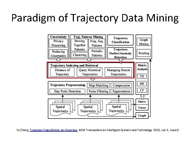
Paradigm of Trajectory Data Mining Yu Zheng. Trajectory Data Mining: An Overview. ACM Transactions on Intelligent Systems and Technology. 2015, vol. 6, issue 3.

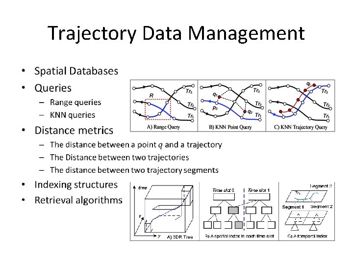
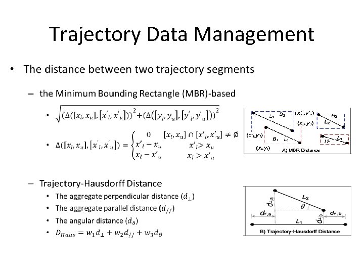
Trajectory Data Management •

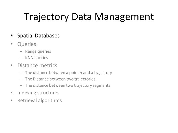
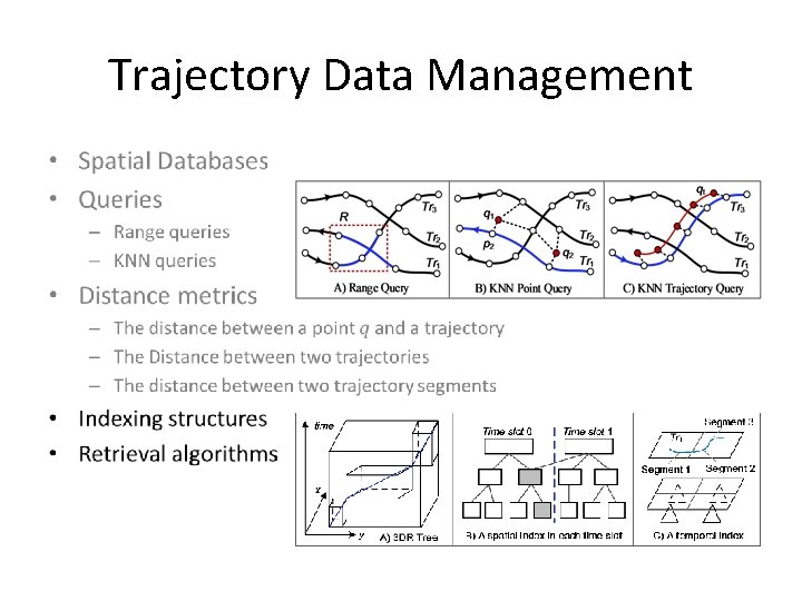
Trajectory Data Management •

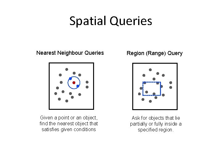
Spatial Queries Nearest Neighbour Queries Given a point or an object, find the nearest object that satisfies given conditions Region (Range) Query Ask for objects that lie partially or fully inside a specified region.

Spatial Indexing Structures • Space Partition-Based Indexing Structures – Grid-based – Quad-tree – k-D tree • Data-Driven Indexing Structures – R-Tree

Spatial Indexing Structures • Space Partition-Based Indexing Structures – Grid-based – Quad-tree – k-D tree • Data-Driven Indexing Structures – R-Tree

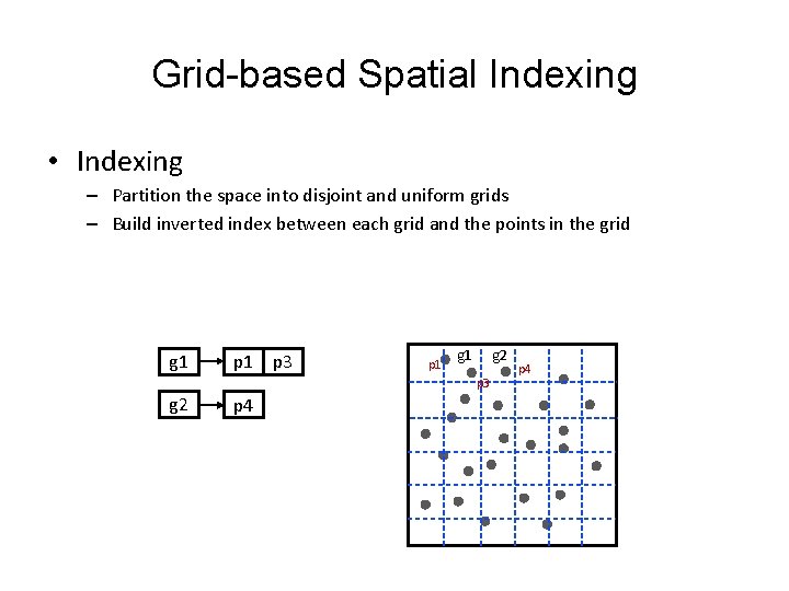
Grid-based Spatial Indexing • Indexing – Partition the space into disjoint and uniform grids – Build inverted index between each grid and the points in the grid g 1 p 3 p 1 g 2 g 1 p 3 g 2 p 4

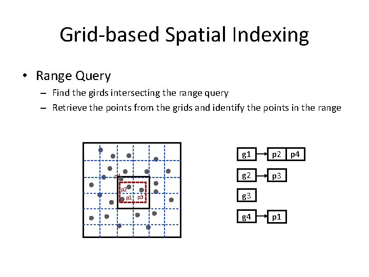
Grid-based Spatial Indexing • Range Query – Find the girds intersecting the range query – Retrieve the points from the grids and identify the points in the range p 4 p 2 p 1 p 3 g 1 p 2 p 4 g 2 p 3 g 4 p 1

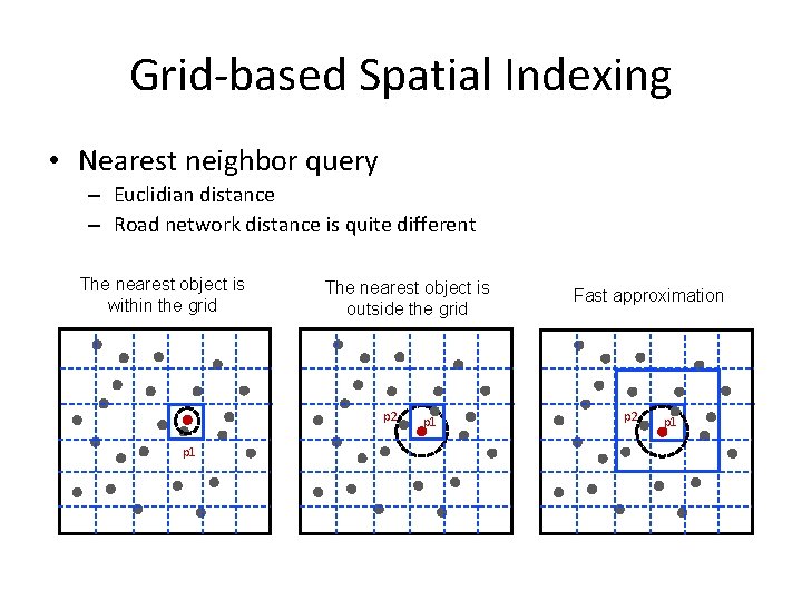
Grid-based Spatial Indexing • Nearest neighbor query – Euclidian distance – Road network distance is quite different The nearest object is within the grid The nearest object is outside the grid p 2 p 1 Fast approximation p 2 p 1

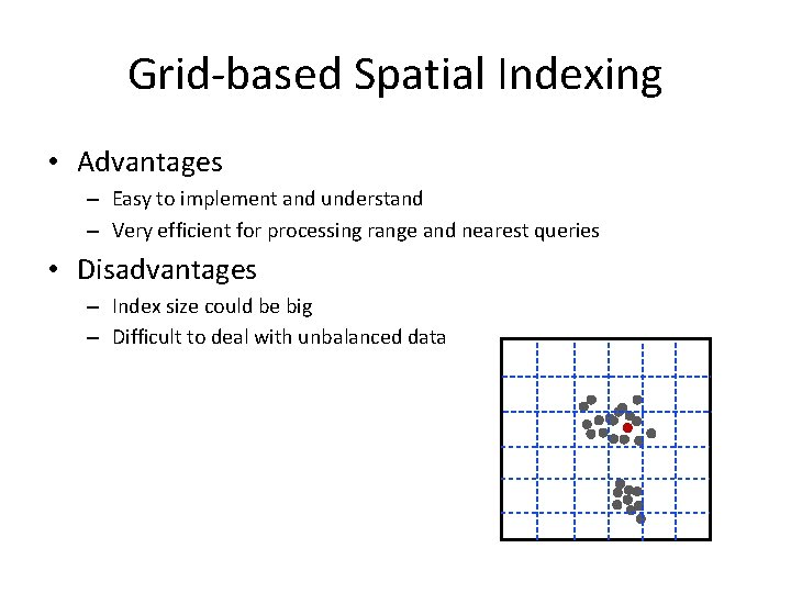
Grid-based Spatial Indexing • Advantages – Easy to implement and understand – Very efficient for processing range and nearest queries • Disadvantages – Index size could be big – Difficult to deal with unbalanced data

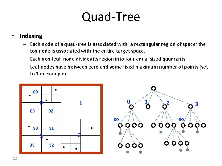
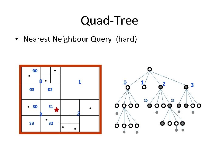
Quad-Tree • Indexing – Each node of a quad-tree is associated with a rectangular region of space; the top node is associated with the entire target space. – Each non-leaf node divides its region into four equal sized quadrants – Leaf nodes have between zero and some fixed maximum number of points (set to 1 in example). 00 0 03 0 1 30 31 2 3 12 2 3 02 00 33 1 32 30

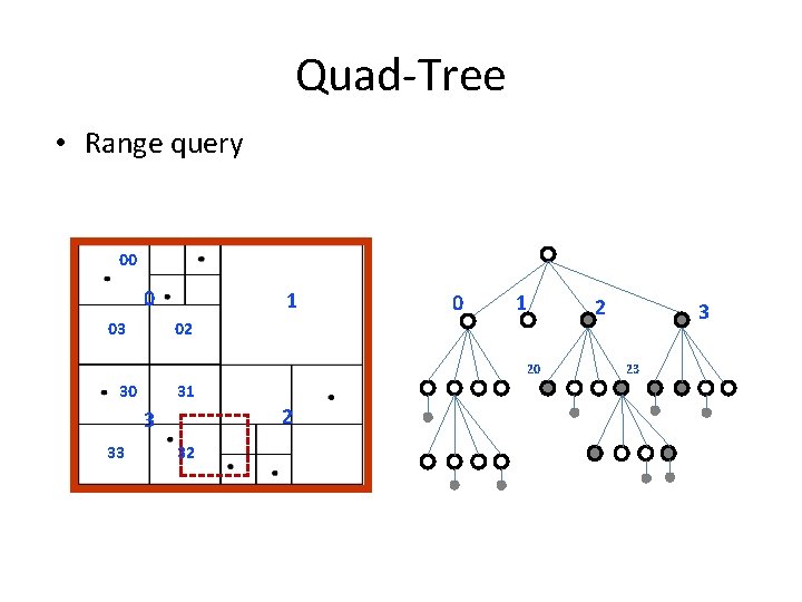
Quad-Tree • Range query 00 0 03 1 02 20 30 31 2 3 33 32 2 3 23

Quad-Tree • Nearest Neighbour Query (hard) 00 0 03 1 02 20 30 31 2 3 33 32 2 3 23

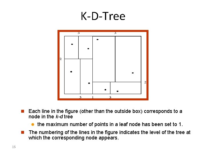
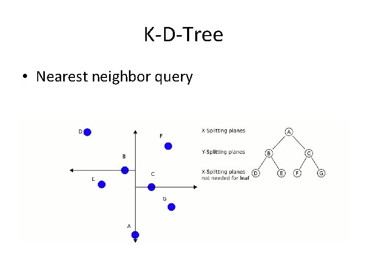
K-D-Tree Each line in the figure (other than the outside box) corresponds to a node in the k-d tree the maximum number of points in a leaf node has been set to 1. The numbering of the lines in the figure indicates the level of the tree at which the corresponding node appears. 15

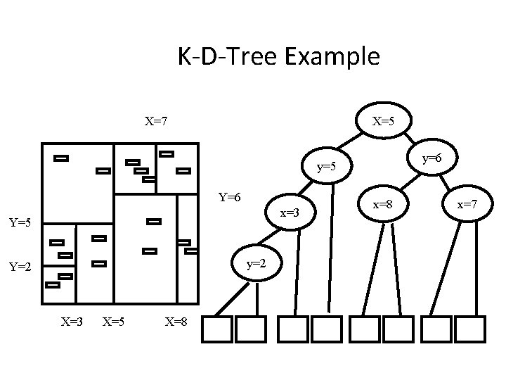
K-D-Tree Example X=7 X=5 y=6 y=5 Y=6 x=3 Y=5 y=2 Y=2 X=3 X=5 X=8 x=7

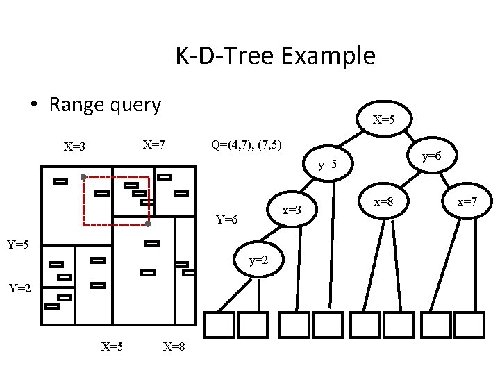
K-D-Tree Example • Range query X=5 X=7 X=3 Q=(4, 7), (7, 5) y=6 y=5 x=3 Y=6 Y=5 y=2 Y=2 X=5 X=8 x=7

K-D-Tree • Nearest neighbor query

Spatial Indexing Structures • Space Partition-Based Indexing Structures – Grid-based – Quad-tree – k-D tree • Data-Driven Indexing Structures – R-Tree

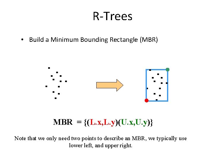
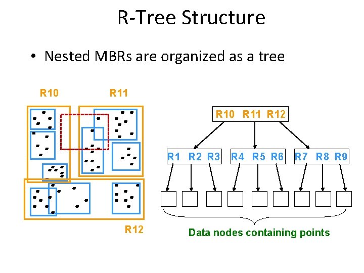
R-Trees • Build a Minimum Bounding Rectangle (MBR) MBR = {(L. x, L. y)(U. x, U. y)} Note that we only need two points to describe an MBR, we typically use lower left, and upper right.

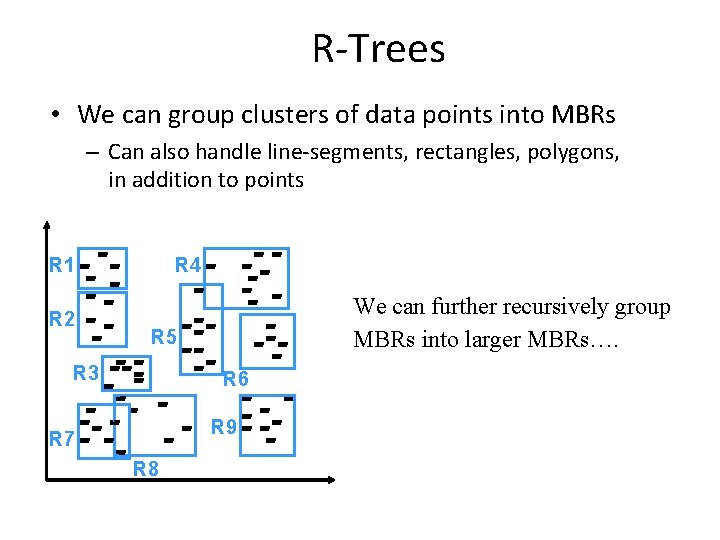
R-Trees • We can group clusters of data points into MBRs – Can also handle line-segments, rectangles, polygons, in addition to points R 1 R 2 R 4 We can further recursively group MBRs into larger MBRs…. R 5 R 3 R 6 R 9 R 7 R 8

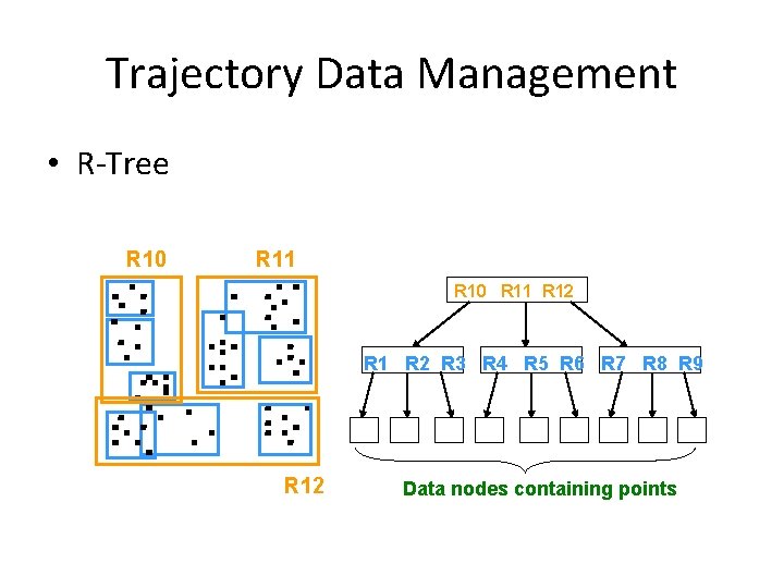
R-Tree Structure • Nested MBRs are organized as a tree R 10 R 11 R 12 R 1 R 2 R 3 R 12 R 4 R 5 R 6 R 7 R 8 R 9 Data nodes containing points

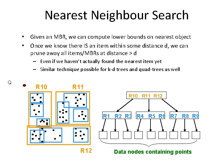
Nearest Neighbour Search • Given an MBR, we can compute lower bounds on nearest object • Once we know there IS an item within some distance d, we can prune away all items/MBRs at distance > d – Even if we haven’t actually found the nearest item yet – Similar technique possible for k-d trees and quad-trees as well Q R 10 R 11 R 12 R 1 R 2 R 3 R 4 R 5 R 6 R 7 R 8 R 9 R 12 Data nodes containing points

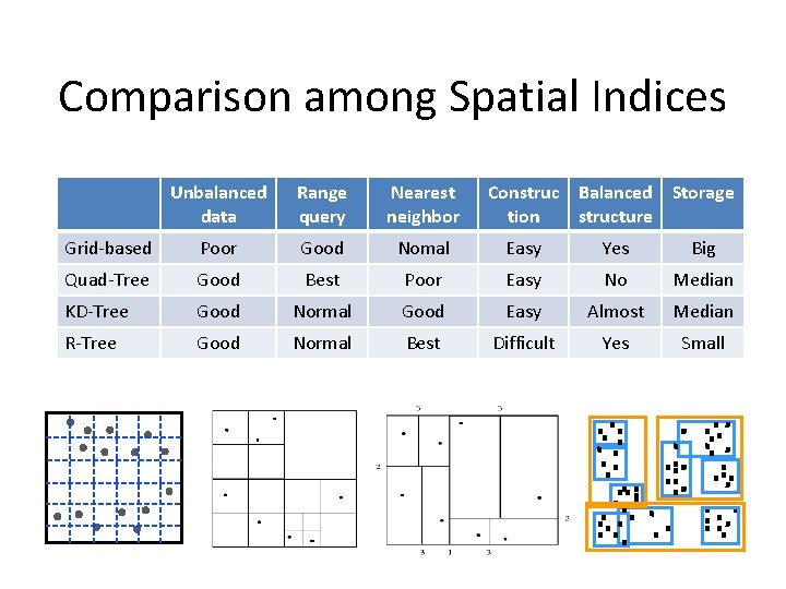
Comparison among Spatial Indices Unbalanced data Range query Nearest neighbor Construc Balanced Storage tion structure Grid-based Poor Good Nomal Easy Yes Big Quad-Tree Good Best Poor Easy No Median KD-Tree Good Normal Good Easy Almost Median R-Tree Good Normal Best Difficult Yes Small

Trajectory Data Management •

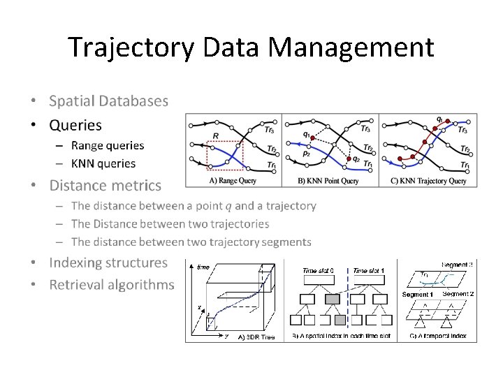
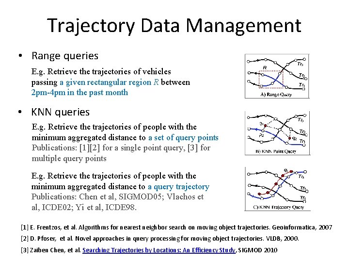
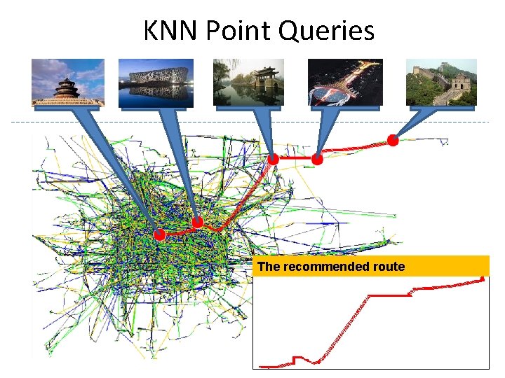
Trajectory Data Management • Range queries E. g. Retrieve the trajectories of vehicles passing a given rectangular region R between 2 pm-4 pm in the past month • KNN queries E. g. Retrieve the trajectories of people with the minimum aggregated distance to a set of query points Publications: [1][2] for a single point query, [3] for multiple query points E. g. Retrieve the trajectories of people with the minimum aggregated distance to a query trajectory Publications: Chen et al, SIGMOD 05; Vlachos et al, ICDE 02; Yi et al, ICDE 98. [1] E. Frentzos, et al. Algorithms for nearest neighbor search on moving object trajectories. Geoinformatica, 2007 [2] D. Pfoser, et al. Novel approaches in query processing for moving object trajectories. VLDB, 2000. [3] Zaiben Chen, et al. Searching Trajectories by Locations: An Efficiency Study, SIGMOD 2010

Trajectory Data Management •

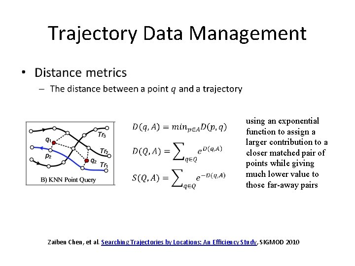
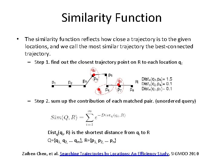
Trajectory Data Management • using an exponential function to assign a larger contribution to a closer matched pair of points while giving much lower value to those far-away pairs Zaiben Chen, et al. Searching Trajectories by Locations: An Efficiency Study, SIGMOD 2010

Trajectory Data Management •

Trajectory Data Management •

Trajectory Data Management •

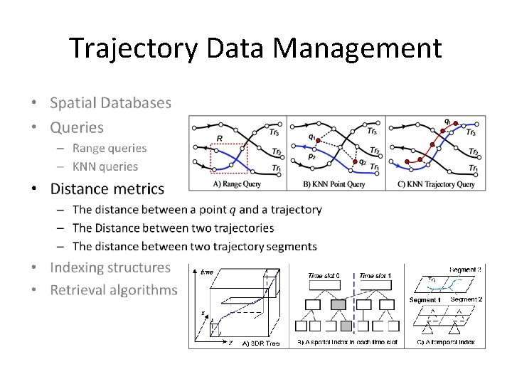
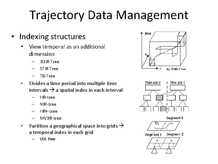
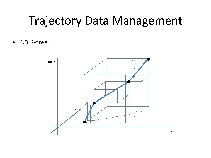
Trajectory Data Management • Indexing structures • View temporal as an additional dimension – – – • Divides a time period into multiple time intervals a spatial index in each interval – – • 3 D R-Tree ST R-Tree TB-Tree HR-tree MR-tree HR+-tree MV 3 R-tree Partition a geographical space into grids a temporal index in each grid – CSE-Tree

Trajectory Data Management • R-Tree R 10 R 11 R 12 R 1 R 2 R 3 R 4 R 5 R 6 R 7 R 8 R 9 R 12 Data nodes containing points

Trajectory Data Management • 3 D R-tree Time y x

Trajectory Data Management • Multi-version R-tree (HR-tree [Tao 2001 a], HR+-tree[Tao 2001 b], MR-tree[Xu 2005]) For each timestamp, an R-tree is created. So, there are many R-trees. These R-trees are indexed. HR-tree [Tao 2001] Query for trajectories in a given region and in a given time interval: 1. The R-tree at the timestamp is found first 2. The trajectories in the specified region are retrieved from the R-tree.

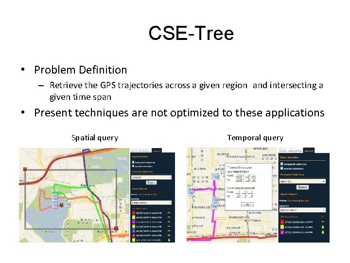
CSE-Tree • Problem Definition – Retrieve the GPS trajectories across a given region and intersecting a given time span • Present techniques are not optimized to these applications Spatial query Temporal query

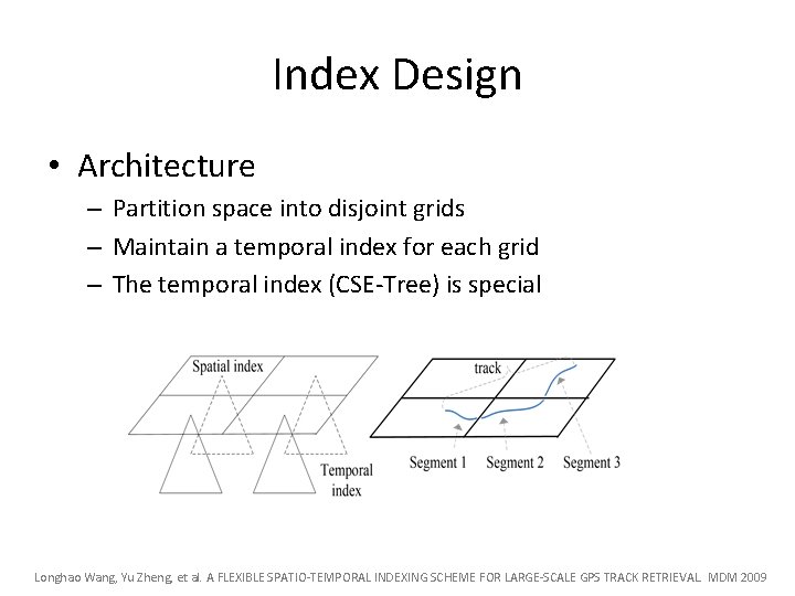
Index Design • Architecture – Partition space into disjoint grids – Maintain a temporal index for each grid – The temporal index (CSE-Tree) is special Longhao Wang, Yu Zheng, et al. A FLEXIBLE SPATIO-TEMPORAL INDEXING SCHEME FOR LARGE-SCALE GPS TRACK RETRIEVAL. MDM 2009

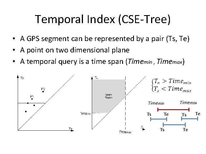
Temporal Index (CSE-Tree) • A GPS segment can be represented by a pair (Ts, Te) • A point on two dimensional plane • A temporal query is a time span (Timemin , Timemax) Timemin Ts Te Ts Timemax Ts Te Te

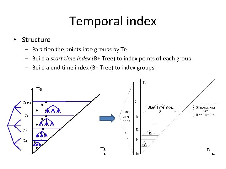
Temporal index • Structure – Partition the points into groups by Te – Build a start time index (B+ Tree) to index points of each group – Build a end time index (B+ Tree) to index groups Te ti+1 ti t 2 t 1 Ts

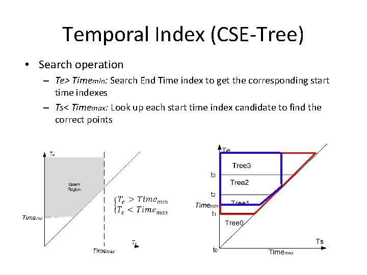
Temporal Index (CSE-Tree) • Search operation – Te> Timemin: Search End Time index to get the corresponding start time indexes – Ts< Timemax: Look up each start time index candidate to find the correct points

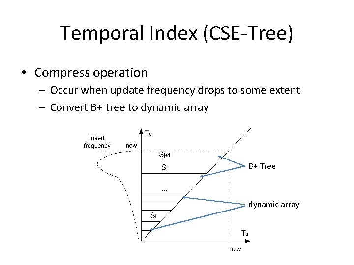
Temporal Index (CSE-Tree) • Compress operation – Occur when update frequency drops to some extent – Convert B+ tree to dynamic array B+ Tree dynamic array

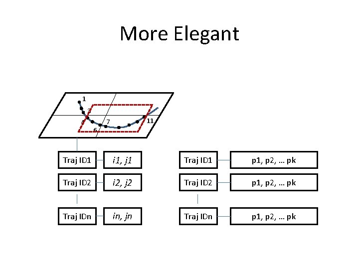
More Elegant 1 3 4 6 11 7 Traj ID 1 i 1, j 1 Traj ID 1 p 1, p 2, … pk Traj ID 2 i 2, j 2 Traj ID 2 p 1, p 2, … pk Traj IDn in, jn Traj IDn p 1, p 2, … pk

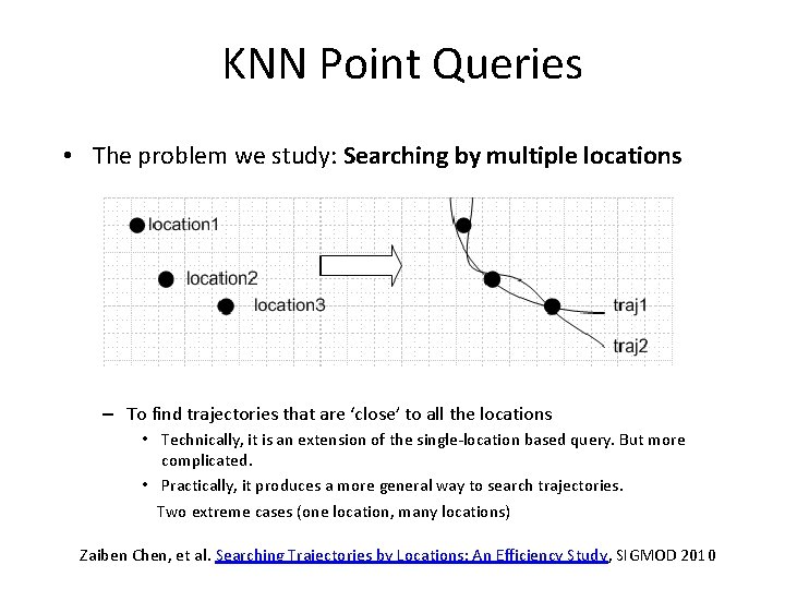
KNN Point Queries • The problem we study: Searching by multiple locations – To find trajectories that are ‘close’ to all the locations • Technically, it is an extension of the single-location based query. But more complicated. • Practically, it produces a more general way to search trajectories. Two extreme cases (one location, many locations) Zaiben Chen, et al. Searching Trajectories by Locations: An Efficiency Study, SIGMOD 2010

KNN Point Queries The recommended route

Similarity Function • The similarity function reflects how close a trajectory is to the given locations, and we call the most similar trajectory the best-connected trajectory. – Step 1. find out the closest trajectory point on R to each location qi – Step 2. sum up the contribution of each matched pair. (unordered query) Distq(qi, R) is the shortest distance from qi to R Q={q 1, q 2, … qm}, R={p 1, p 2, … pn} Zaiben Chen, et al. Searching Trajectories by Locations: An Efficiency Study, SIGMOD 2010

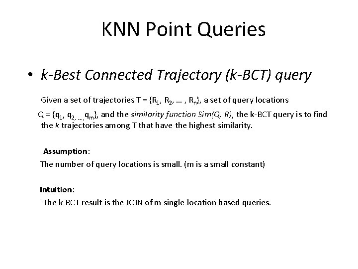
KNN Point Queries • k-Best Connected Trajectory (k-BCT) query Given a set of trajectories T = {R 1, R 2, … , Rn}, a set of query locations Q = {q 1, q 2, … , qm}, and the similarity function Sim(Q, R), the k-BCT query is to find the k trajectories among T that have the highest similarity. Assumption: The number of query locations is small. (m is a small constant) Intuition: The k-BCT result is the JOIN of m single-location based queries.

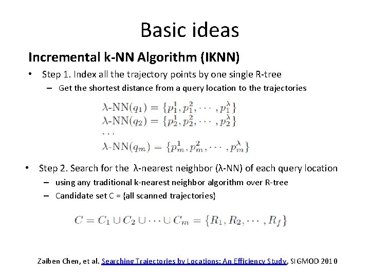
Basic ideas Incremental k-NN Algorithm (IKNN) • Step 1. Index all the trajectory points by one single R-tree – Get the shortest distance from a query location to the trajectories • Step 2. Search for the λ-nearest neighbor (λ-NN) of each query location – using any traditional k-nearest neighbor algorithm over R-tree – Candidate set C = {all scanned trajectories} Zaiben Chen, et al. Searching Trajectories by Locations: An Efficiency Study, SIGMOD 2010

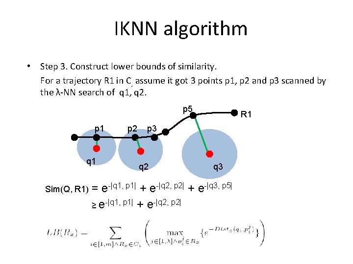
IKNN algorithm • Step 3. Construct lower bounds of similarity. For a trajectory R 1 in C, assume it got 3 points p 1, p 2 and p 3 scanned by the λ-NN search of q 1, q 2. p 5 p 1 q 1 Sim(Q, R 1) = p 2 R 1 p 3 q 2 q 3 e-|q 1, p 1| + e-|q 2, p 2| + e-|q 3, p 5| ≥ e-|q 1, p 1| + e-|q 2, p 2|

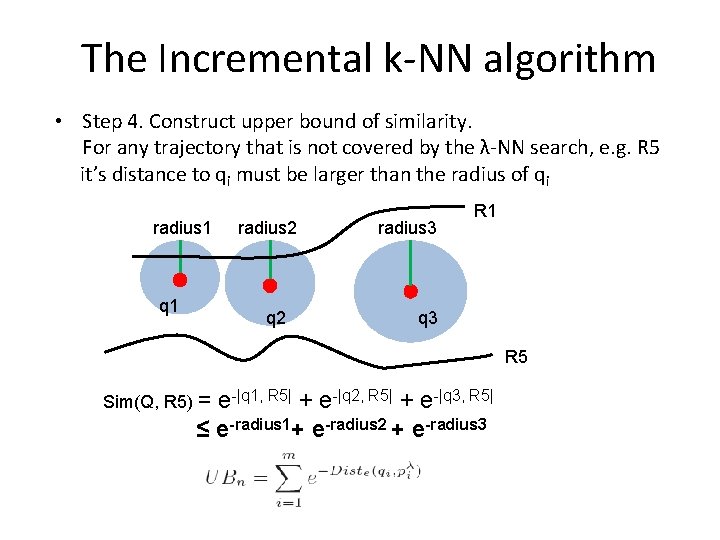
The Incremental k-NN algorithm • Step 4. Construct upper bound of similarity. For any trajectory that is not covered by the λ-NN search, e. g. R 5 it’s distance to qi must be larger than the radius of qi radius 1 q 1 radius 2 q 2 radius 3 R 1 q 3 R 5 Sim(Q, R 5) = e-|q 1, R 5| + e-|q 2, R 5| + e-|q 3, R 5| ≤ e-radius 1+ e-radius 2 + e-radius 3

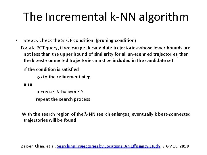
The Incremental k-NN algorithm • Step 5. Check the STOP condition (pruning condition) For a k-BCT query, if we can get k candidate trajectories whose lower bounds are not less than the upper bound of similarity for all un-scanned trajectories, then the k best-connected trajectories must be included in the candidate set. if the condition is satisfied go to the refinement step else increase λ by some Δ repeat the search process With the search region of the λ-NN search enlarges, eventually k best-connected trajectories will be found Zaiben Chen, et al. Searching Trajectories by Locations: An Efficiency Study, SIGMOD 2010

Thanks! Yu Zheng yuzheng@microsoft. com Homepage Yu Zheng. Trajectory Data Mining: An Overview. ACM Transactions on Intelligent Systems and Technology. 2015, vol. 6, issue 3.