Traffic grooming in WDM Networks Dynamic Traffic Grooming

Traffic grooming in WDM Networks • Dynamic Traffic Grooming in WDM Mesh Networks Using a Novel Graph Model by Hongyue Zhu, Hui Zang, Keyao Zhu, and Biswanath Mukherjee

What is Traffic Grooming? • When low speed traffic streams are multiplexed and switched onto high-speed light paths, we say traffic is groomed. • Grooming is mainly done to reduce the no of Add Drop Multiplexers (ADM) required. As they are major contributors to the total cost.

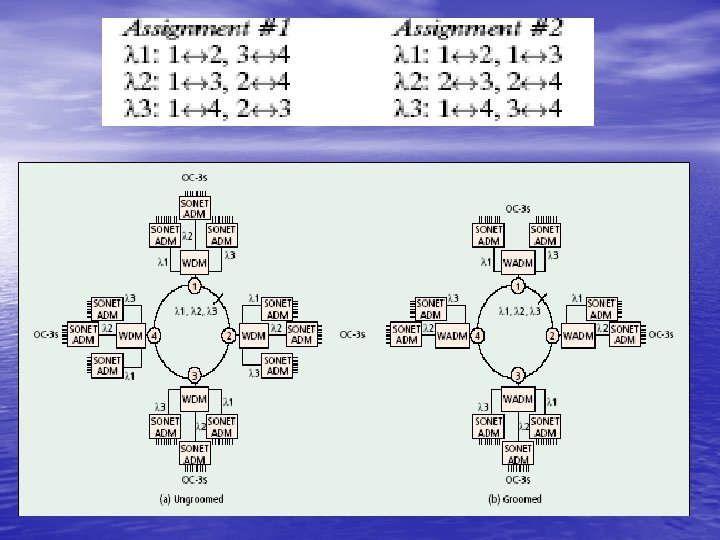
Motivation for Traffic Grooming • Suppose that each wavelength is used to support an. OC-48 ring, and that the traffic requirement is for eight OC-3 circuits between each pair of nodes. In this example we have six node pairs, and the total traffic load is equal to 48 OC-3 s or equivalently three OC-48 rings. In the next slide 2 possible assignments are shown.

Motivation for Traffic Grooming (cond. . ) • Thus we can see that by careful selection of wavelengths passing through a node we can reduce the required no of ADM’S. • Application of RAW alone does not imply that the solution selected is optimal in no of ADM’S required. Consider the example on the next slide.

• As shown RAW 1 requires only 2 wavelengths and 15 AMD’S. While RAW 2 requires 3 wavelengths , but consume only 9 AMD’S. • Generally a traffic grooming problem can be formulated as an ILP. But as the network size grows the no of equations and variables increase explosively.

Novel Graph Model • Auxiliary graph: Captures various network • constrains, like no of transceivers at each node, no of wavelengths on each fiber-link, wavelength -conversion capabilities of each node etc (will be discussed in details) Dynamic traffic grooming Algorithm: This is a route computing algorithm, which take the weight function into account. Thus by dynamically adjusting the weight’s on the edges, one could evolve from one grooming policy to another, as demand changes.

Construction of an Auxiliary Graph • Consider a network of 3 nodes • Each link has two wavelengths • All nodes are assumed to have grooming • • • functionality Node 0 has full wavelength-conversion Node 1 has no wavelength-conversion Node 2 has limited wavelength-conversion capability (i. e. wavelength 1 can be converted to wavelength 2)

Construction of an Auxiliary Graph (cond. . ) • Auxiliary graph is a layered graph with w+2 layers, where w = no of wavelengths • W+1 layer is called the Light path Layer • W+2 layer is called the Access layer. • Each node layer has 2 vertices input (I) and output (o).

Construction of an Auxiliary Graph (cond. . ) Meaning of Edges • Wavelength Bypass Edges (WBE). There is an edge from • • the input port to the output port on each wavelength layer l at node i, denoted as WBE (i, l). Grooming Edges (Grm. E). There is an edge from the input port to the output port on access layer at node I if node i has grooming capability, denoted as Grm. E (i). Mux Edges (Mux. E). There is an edge from the output port on the access layer to the output port on the lightpath layer at each node, denoted as Mux. E(i).

Construction of an Auxiliary Graph (cond. . ) Meaning of Edges • Demux Edges (Dmx. E). There is an edge from • the input port on the lightpath layer to the input port on the access layer at each node, denoted as Dmx. E (i). Transmitter Edges (Tx. E). There is an edge from the output port on the access layer to the output port on wavelength layer l, denoted as Tx. E(i, l), if there are transmitters available on wavelength λi at node i.

Construction of an Auxiliary Graph (cond. . ) Meaning of Edges • Receiver Edges (Rx. E). There is an edge from the • input port on wavelength layer l to the input port on the access layer, denoted as Rx. E(i, l), if there are receivers available on wavelength λi at node i. Converter Edges (Cvt. E). There is an edge from the input port on wavelength layer l 1 to the output port on wavelength layer l 2 at node i, denoted as Cvt. E(i, l 1, l 2), if wavelength l 1 can be converted to wavelength l 2 at node i.

Construction of an Auxiliary Graph (cond. . ) Meaning of Edges • Wavelength-Link Edges (WLE). There is an edge • from the output port on wavelength layer l at node i to the input port on wavelength layer l at node j, denoted as WLE(i, j, l), if there is a physical link from node i to node j and wavelength λl on this link is not used. Lightpath Edges (LPE). There is an edge from the output port on the lightpath layer at node i to the input port on the lightpath layer at node j, denoted as LPE(i, j), if there is a lightpath from node i to node j.

Construction of an Auxiliary Graph (cond. . ) – Each edge is associated with the tuple P(c, w). – For wavelength-link edges c = capacity of the corresponding wavelength on the corresponding link. – For lightpath edges c = residual capacity of corresponding lightpath. – For all other type of edges c = infinity. – Weight w reflect cost of element. – Weights can be fixed of adjusted in accordance to network state – Fixed weight Fixed grooming policy – Variable weight Adaptive grooming policy

Auxiliary Graph

Dynamic traffic grooming Algorithm • 1. 2. Inputs: Initial network state Set of traffic demands represented as T (s, d, g, m). s = source, d= destination, g= granularity of traffic and m = amount of traffic in g units.

Algorithm steps • Initialize: Construct auxiliary graph. • When request T arrives 1 Compute the shortest path p from the output port on the access layer of the source to the input port on the access layer of the destination of T on graph G, ignoring the edges whose capacities are less than the requirement of the request. If such a path does not exist, block the traffic demand; otherwise, continue with the following steps.

Algorithm steps 2 If p contains wavelength-link edges, set up one or more lightpaths going through the corresponding wavelength-links. 3 Route T along the pre-existing lightpaths in p and/or lightpaths newly set up according to p. 4 Update graph G as follows:

Algorithm steps • For each newly setup lightpath, a • lightpath edge from the output port of the starting node of the lightpath to the input port of the ending node of the lightpath is added on the lightpath layer. The wavelength-link edges used by the lightpath are removed from the corresponding wavelength layers.

Algorithm steps • If there is no more transmitter/receiver available • • at node i on wavelength λl , the corresponding transmitter/receiver edge will be removed from G, i. e. , this node cannot source/sink a lightpath on wavelength λl any more and can only be bypassed by a lightpath. If there is no more wavelength converter which can convert wavelength l 1 to wavelength l 2 available at node i, the converter edge will be removed from G. Update tuple P(c, w)

Algorithm steps 5 If connection removed A Remove the traffic from network. B Tear down all the lightpaths C Update graph G by applying reverse of update methods used in step 4 above.

Example • Assume: • Capacity of each wavelength = OC-48 • Each node has grooming capability and two tunable transceivers. • First connection request = T(1, 0, OC-12, 2) Path found : TXE(1, 1) WLE(1, 0, 1) and RXE(0, 1) LPE(0, 1) = 24

Example

Example • Another request: T(2, 0, OC-12, 1) Path found: • Case 1: Tx. E(2, 2), WLE(2, 1, 2), WBE(1, 2), WLE(1, 0, 2), and Rx. E(0, 2) LPE(2, 0) = 36 LPE(1, 0) = 24 • Case 2: Tx. E(2, 1), WLE(2, 1, 1), Rx. E(1, 1), Grm. E(1), Mux. E(1), LPE(1, 0), and Dmx. E(0) LPE(2, 1) = 36 AND LPE(1, 0) = 12

case 1

Case 2

Grooming Operations • Op 1: Route the traffic onto an existing lightpath Op 1: • • directly connecting the source s and the destination d. Op 2: Route the traffic through multiple existing lightpaths. Op 3: Set up a new lightpath directly between the source s and the destination d and route the traffic onto this lightpath. Using this operation, we set up only one lightpath if the amount of the traffic is less than or equal to the capacity of the lightpath.

Grooming Operations • Op 4: Set up one or more lightpaths that do not directly connect source s and destination d, and route the traffic onto these lightpaths and/or some existing lightpaths. Using this operation, we need to set up at least one new lightpath. However, since some existing lightpaths may be utilized, the number of wavelength-links used to set up the new lightpaths could be less than the number of wavelength-links needed to set up a lightpath directly connecting source s and destination d.

Grooming Policies • By combining various grooming operations in different priority order , we can achieve different grooming policies 1. Minimize the Number of Traffic Hops on the Virtual Topology (Min. THV) : This policy chooses the route with the fewest lightpaths for a connection. 2. Minimize the Number of Traffic Hops on the Physical Topology (Min. THP) : We compare the number of wavelength-links used by all the four operations and choose the one with the fewest wavelength-links.

Grooming Policies 3. Minimize the Number of Lightpaths (Min. LP) : This policy is similar to Min. THV but it tries to set up the minimal number of new lightpaths to carry the traffic. 4. Minimize the Number of Wavelength-Links (Min. WL) : This policy is similar to Min. THP but it tries to consume the minimum number of extra wavelength-links, i. e. , wavelength-links not being used by any lightpaths for now, to carry the traffic

Dominant edge • if a path p 1 in the graph contains more of this kind of • • edges than another path p 2, then the weight of p 1 is always larger than that of p 2. Here, the weight of a path is the summation of the weights of the edges it traverses. Example: To achieve Min. THV, we just need to make Grm. Es the dominant edges. To achieve Min. LP, we should make Tx. Es and Rx. Es the dominant edges. To achieve Min. WL, WLEs should be the dominant edges

Results

Results

Adaptive grooming policy • Since Min. THV performs best when transceivers are the more constrained resources and Min. THP gives the best results when wavelength-links become more scarce resources, Adaptive Grooming Policy (AGP) take advantages of both these policies and performs well over all network conditions.

Adaptive grooming policy • ratio of the number of unused wavelength-links in the network to the total number of available transceivers at all nodes as an indicator of the network state. If the ratio is larger than the set threshold d 1 then Min. THV will be used and if the ratio is less that the set threshold d 2 then Min. THP will be used. If ratio is in between the policy is not changed.

Adaptive grooming policy

Adaptive grooming policy

Conclusion • The new model takes various constrains into account and can achieve various objectives by using different grooming policies. The ability to adjust grooming policy by changing the weights of the edges makes this model very suitable for dynamic traffic grooming.