Traffic Flow Fundamentals CE 331 Transportation Engineering Objectives

Traffic Flow Fundamentals CE 331 Transportation Engineering

Objectives Understand the fundamental relationships among traffic parameters ¢ Estimating traffic parameters using the fundamental relationship ¢ Queuing Models ¢ 2
 l ¢ Density (k) l ¢ Rate of traffic")
Some Terms ¢ Speed (u) l ¢ Density (k) l ¢ Rate of traffic over distance (vpm) Volume (V) l ¢ Rate of motion (mph) Amount of traffic (vph) Flow (q) l Rate of traffic (vph); equivalent hourly rate

Basic Relationships Low volumes Highest speeds High volumes Lower speeds Highest volumes Maximum density Medium density No speed or flow q=ku

Basic Relationships 5

Flow-Density Example If the spacing between vehicles is 500 feet what is the density? d = 1/k k = 1/d = 1 veh/500 feet = 0. 002 vehicles/foot = 10. 6 veh/mile

Speed-Density Relationship Max speed 0 density uf Speed Max density 0 speed Density 7 kj

Speed-Density Relationship 8

Flow-Density Relationship Optimum density qcap kcap 9 kj Density

Flow-Density Relationship 10
 B Slope of these lines is the space mean")
Flow – density (and speed) B Slope of these lines is the space mean speed at this density KB Do the dimensional analysis

Flow-Density Example If the space mean speed is 45. 6 mph, what is the flow rate? q = kus = (10. 6 veh/mile)(45. 6 mph) = 481. 5 veh/hr

Speed-Flow Relationship uf “Optimal” speed for flow maximization ucap qcap= kcapucap qcap 13 Flow

Speed-Flow Relationship 14

Highway capacity manual Source 1985 highway capacity manual

2000 Highway Capacity Manual

Speed density relationship Capacity Drop Source: Maze, Schrock, and Van. Der. Horst, “Traffic Management Strategies for Merge Areas in Rural Interstate Work Zones
 uf ucap qcap 18 kcap kj")
Speed-Flow-Density Relationship (Greenshield’s Linear Model) uf ucap qcap 18 kcap kj
 When Greenshield’s Model holds,")
Special Case ¢ Greenshield’s Model l ¢ 19 Linear (Only) When Greenshield’s Model holds,

Greenshield Linear Model

Example 1 A highway section has an average spacing of 25 ft under jam conditions and a freeflow speed of 55 mph. Assuming that the relationship between speed and density is linear, determine the jam density, the maximum flow, the density at maximum flow, and the speed at maximum flow. 21

Example 2 Traffic observations along a freeway lane showed the flow rate of 1200 vph occurred with an average speed of 50 mph. The same study also showed that the free-flow speed is 60 mph and the speed-density relationship follows the Greenshield’s model. What is the capacity of this lane? 22

Example 3 A section of highway is known to have a free-flow speed of 55 mph and a capacity of 3300 vph. In a given hour, 2100 vehicles were counted at a point along the road. If Greenshield’s model applies, what would be the space mean speed of these 2100 vehicles? 23

Queuing Theory The theoretical study of waiting lines, expressed in mathematical terms input server queue Delay= queue time +service time output
 queues Deterministic queuing l Steady state")
Queuing theory ¢ Common ways to represent (model) queues Deterministic queuing l Steady state queuing l Shock waves l
. ¢ We look at steady state: after")
Common Assumptions The queue is FCFS (FIFO). ¢ We look at steady state: after the system has started up and things have settled down. ¢ (all the information necessary to completely describe the system)

Typical cases where queuing is important ¢ Bottle necks – capacity reductions Lane closures for work zones on multilane facilities l Toll booths l Where else would we experience a line in traffic? l

Deterministic queuing model ¢ ¢ Treats the bottle neck like a funnel Assumptions l l Constant headways through out analysis period – what does this imply about density? Capacity does not vary with traffic flow variable (speed, density or flow)

Deterministic queuing treats the waiting line as if it has no length

Deterministic queuing example Example – Suppose we have a lane closure on a freeway and the single lane capacity at the closure is 1, 400 vehicle per hour. Assume that during the first hour we expect the traffic volume of 2, 000 vehicles per hour for one hour and then the volume to reduce to 800 vehicle per hour. At the peak, how long will the queue be and how long will it take to dissipate? Draw a queuing diagram (cumulative arrivals on Y axis, time on X axis)

Deterministic queuing model example

Deterministic queuing traffic signal case

Diagram for traffic signal
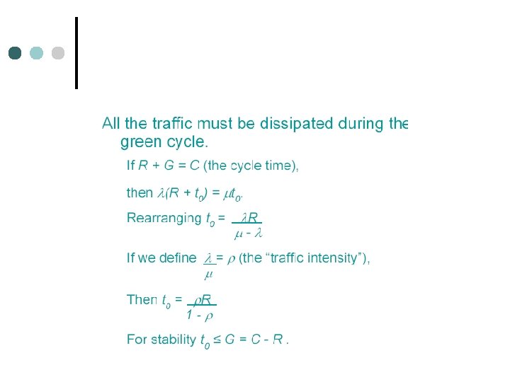

Example λ R µ t 0

Example

Calculating Delay = Average Delay

Intersection delay in both directions

Multiple directions

Minimizing delay

Steady State Queuing ¢ Arrival Distribution l ¢ Service Method l ¢ ¢ Usually first come first serve Service Distribution l ¢ Described by a Poisson distribution Follows a negative exponential distribution Number of channels Assumption of steady state l Average arrival rate is less than average service rate

The M/M/1 System Poisson Process Exponential server queue output

Steady state queuing equation variables • Variables q = Average arrival rate Q = Average service rate n = Number of entities in the system w = Time waiting in the queue v = Time in the system

Arrivals follow a Poisson process n Readily amenable for analysis n Reasonable for a wide variety of situations ¢ a(t) = # of arrivals in time interval [0, t] ¢ q = mean arrival rate ¢ 0 = small time interval Pr(exactly 1 arrival in [t, t+ ]) = q Pr(no arrivals in [t, t+ ]) = 1 -q Pr(more than 1 arrival in [t, t+ ]) = 0 Pr(a(t) = n) = e-q t (q t)n/n!

Model for Interarrivals and Service times · Customers arrive at times t 0 < t 1 <. . - Poisson distributed · The differences between consecutive arrivals are the interarrival times : n = tn - t n-1 · n in Poisson process with mean arrival rate exponentially distributed, q, are Pr( n t) = 1 - e-q t o Service times are exponentially distributed, with Q: Pr(Sn s) = 1 - e-Qs mean service rate

System Features ¢ arrival times are independent service times are independent of the arrivals ¢ Both inter-arrival and service times are memoryless ¢ Pr(Tn > t 0+t | Tn> t 0) = Pr(Tn t) future events depend only on the present state This is a Markovian System

Example of where assumptions are violated 4 -way Stop Arrivals are not random 2 -way Stop

Common one channel equations Example – suppose that cars take an average of 5 seconds at a stop sign. If 9 cars per minute arrive at the sign what is the probability of having 5 in the system what is the probability of having five or fewer. P(5) P(4) P(3) P(2) P(1) P(0) = = = (9/12)5(1 -9/12) = 0. 06 0. 08 0. 11 0. 14 0. 19 0. 25 0. 83

Common queuing equations Expected number of vehicles in the system Expected number of Vehicles in the queue

Common queuing equations Average wait in the queue Average wait in the system

Common queuing equations Probability of spending less than time t in the system Probability of spending less than time t in the queue

Common queuing equations Probability of having more than n vehicles in the system

Shock wave theory ¢ Recognizes that density is a variable l Recognizes the dynamics of the traffic flow Considers non-steady state condition ¢ More realistically represents traffic flow ¢

Example shock wave

Flow – density and speed B KB Slope of these lines is the space mean speed at this density

Back Ward Moving Shock wave Speed of the Shock wave

Example Suppose you have 2, 000 vehicle per hour approaching a lane closure at and average speed of 65 mph. The capacity of the lane closure is 1, 400 vehicles per hour and at the maximum capacity move at 20 mph. Assuming the approaching vehicles are evenly distributed between the two lanes. How fast is the shock wave traveling backwards? Q 1 = 2, 000 vehicles per hour K 1 = 1, 000 per lane per hour/65 mph = 15. 38 vehicles per mile Q 2 = 1, 400 vehicles per hour K 2 = 1, 400 per lane per hour/20 mph = 70 vehicles per mile How fast would the shock wave move backwards if all vehicle approach in a single lane?

Forward moving shock wave
- Slides: 58