TRAFFIC FLOW FORECASTING ON HIGHWAYS EVALUATION AND COMPARISON

TRAFFIC FLOW FORECASTING ON HIGHWAYS EVALUATION AND COMPARISON OF COMMON APPROACHES Hao Peng

Research Questions and Challenges ■ Data collection – Storage – Missing value imputation – What types of data to collect ■ Data analytics – Historical data – Predicative analytics – Real-time forecasting – Video/image analytics

Benefits of Research ■ Intelligent Transportation Systems ■ Road expansion ■ Traffic Apps developers ■ Everyday commuters/travelers

Contributions ■ To evaluate the effectiveness of commonly used statistical and machine learning models on univariate traffic flow forecasting using large amounts of temporal data ■ To study the impacts of incorporating spatially dependent data into multivariate forecasting models ■ To examine the performance of multi-step forecasts and the impacts of varying data resolutions ■ To explore the various trade-offs/pros and cons of the models in terms of accuracy, stability, computational cost, and ease of use

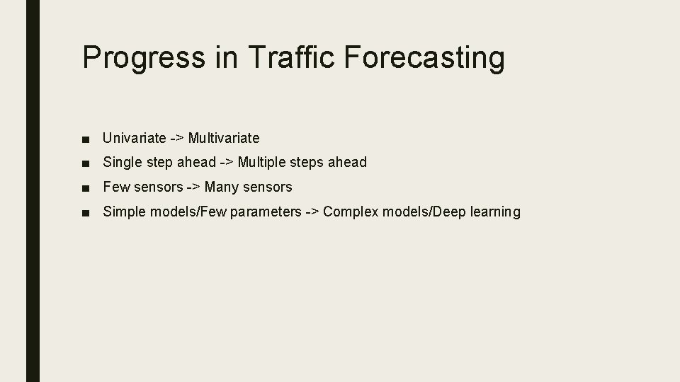
Progress in Traffic Forecasting ■ Univariate -> Multivariate ■ Single step ahead -> Multiple steps ahead ■ Few sensors -> Many sensors ■ Simple models/Few parameters -> Complex models/Deep learning

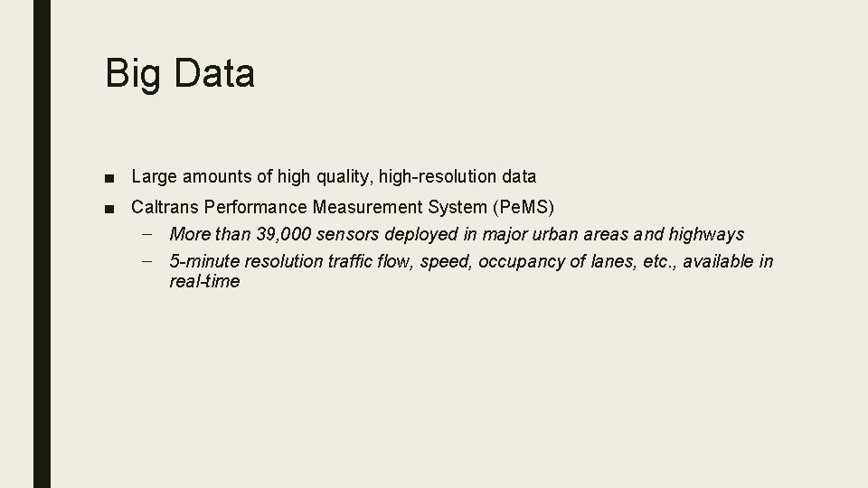
Big Data ■ Large amounts of high quality, high-resolution data ■ Caltrans Performance Measurement System (Pe. MS) – More than 39, 000 sensors deployed in major urban areas and highways – 5 -minute resolution traffic flow, speed, occupancy of lanes, etc. , available in real-time

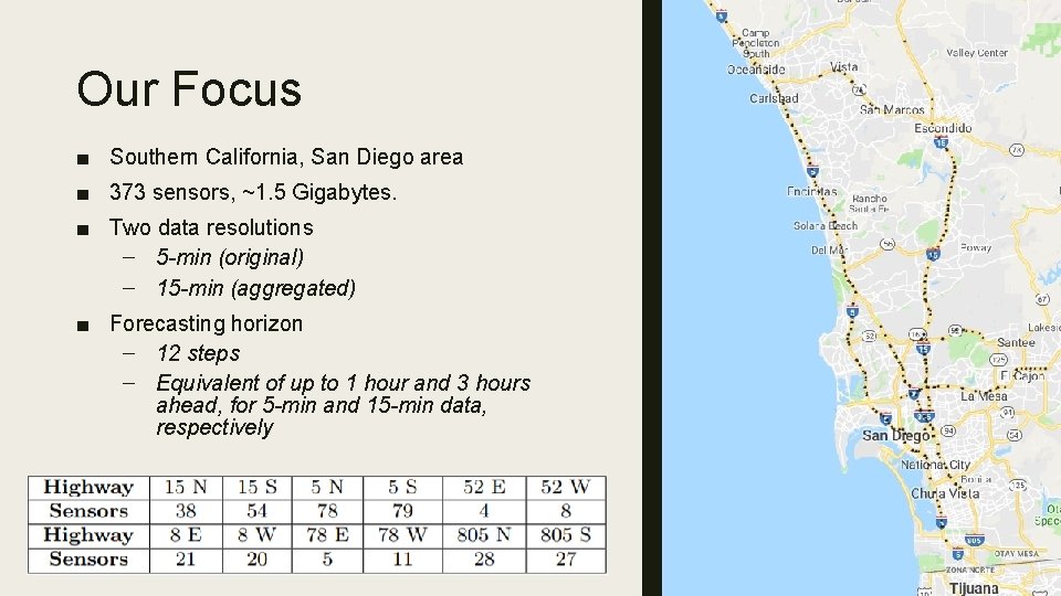
Our Focus ■ Southern California, San Diego area ■ 373 sensors, ~1. 5 Gigabytes. ■ Two data resolutions – 5 -min (original) – 15 -min (aggregated) ■ Forecasting horizon – 12 steps – Equivalent of up to 1 hour and 3 hours ahead, for 5 -min and 15 -min data, respectively

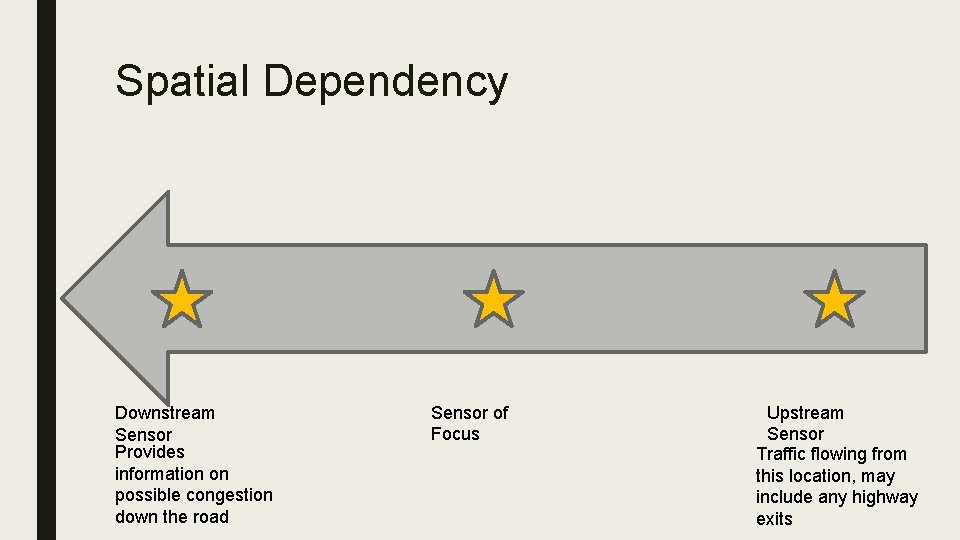
Spatial Dependency Downstream Sensor Provides information on possible congestion down the road Sensor of Focus Upstream Sensor Traffic flowing from this location, may include any highway exits

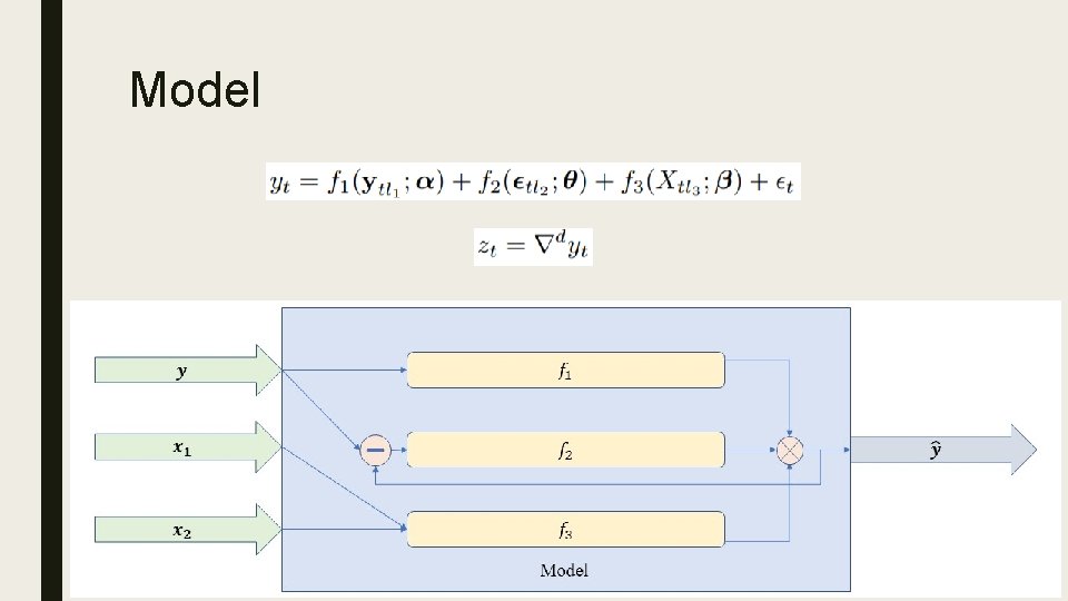
Model

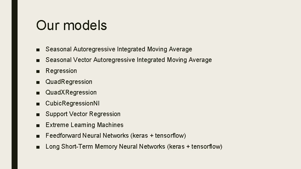
Our models ■ Seasonal Autoregressive Integrated Moving Average ■ Seasonal Vector Autoregressive Integrated Moving Average ■ Regression ■ Quad. XRegression ■ Cubic. Regression. NI ■ Support Vector Regression ■ Extreme Learning Machines ■ Feedforward Neural Networks (keras + tensorflow) ■ Long Short-Term Memory Neural Networks (keras + tensorflow)

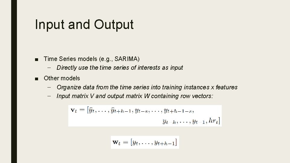
Input and Output ■ Time Series models (e. g. , SARIMA) – Directly use the time series of interests as input ■ Other models – Organize data from the time series into training instances x features – Input matrix V and output matrix W containing row vectors:

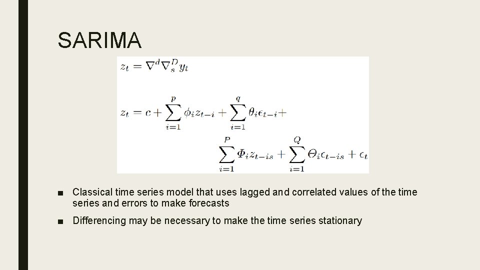
SARIMA ■ Classical time series model that uses lagged and correlated values of the time series and errors to make forecasts ■ Differencing may be necessary to make the time series stationary

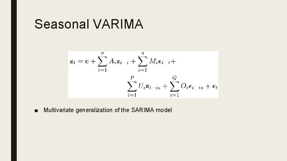
Seasonal VARIMA ■ Multivariate generalization of the SARIMA model

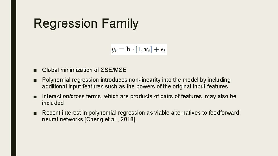
Regression Family ■ Global minimization of SSE/MSE ■ Polynomial regression introduces non-linearity into the model by including additional input features such as the powers of the original input features ■ Interaction/cross terms, which are products of pairs of features, may also be included ■ Recent interest in polynomial regression as viable alternatives to feedforward neural networks [Cheng et al. , 2018].

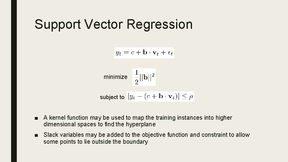
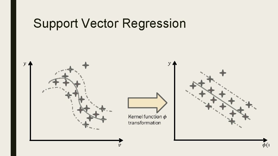
Support Vector Regression minimize subject to ■ A kernel function may be used to map the training instances into higher dimensional spaces to find the hyperplane ■ Slack variables may be added to the objective function and constraint to allow some points to lie outside the boundary

Support Vector Regression

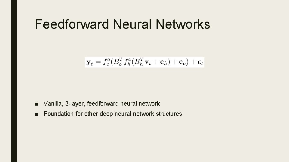
Feedforward Neural Networks ■ Vanilla, 3 -layer, feedforward neural network ■ Foundation for other deep neural network structures

Extreme Learning Machine ■ A special type of feedforward neural network, as follows – Input-to-Hidden: apply activation function to inputs with fixed, random weights. This introduces non-linearity into the data. – Hidden-to-Output: use linear regression to learn the outputs from the hidden features. ■ Compared with a standard feedforward neural network, ELM requires minimal parameter tuning and much lower computational costs.

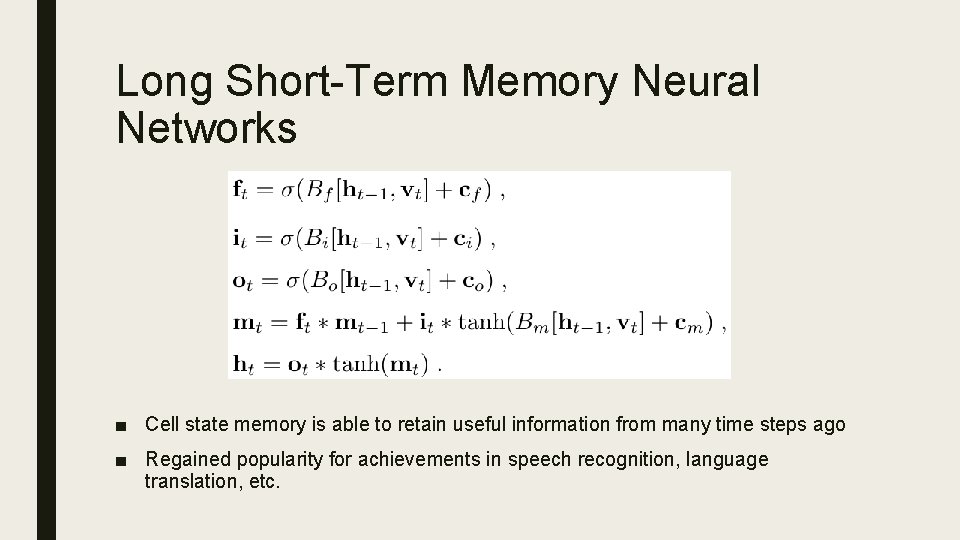
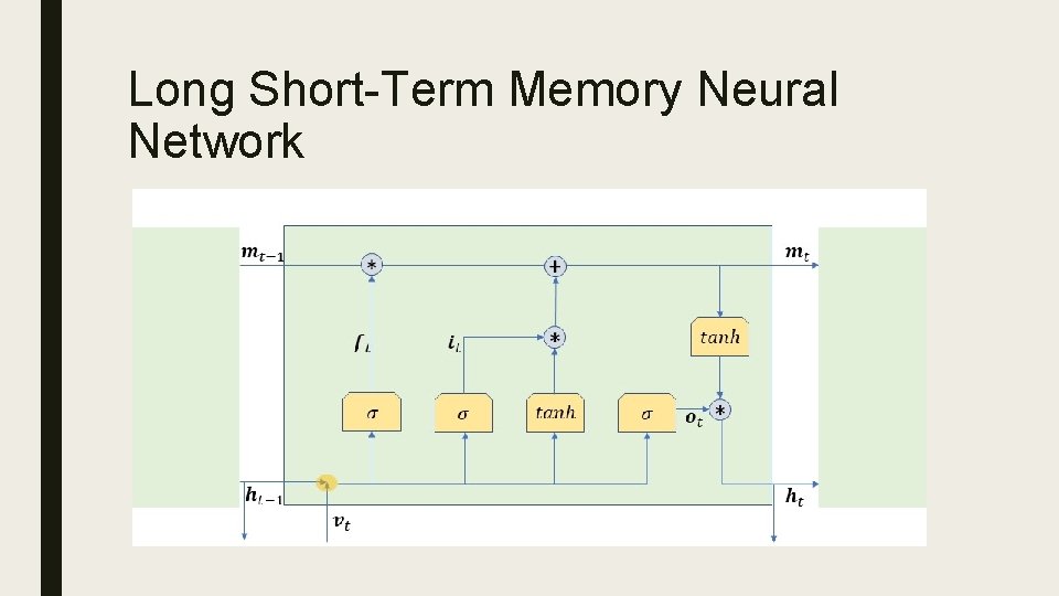
Long Short-Term Memory Neural Networks ■ Cell state memory is able to retain useful information from many time steps ago ■ Regained popularity for achievements in speech recognition, language translation, etc.

Long Short-Term Memory Neural Network

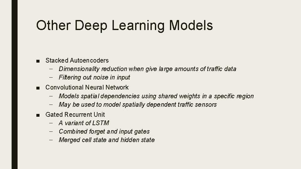
Other Deep Learning Models ■ Stacked Autoencoders – Dimensionality reduction when give large amounts of traffic data – Filtering out noise in input ■ Convolutional Neural Network – Models spatial dependencies using shared weights in a specific region – May be used to model spatially dependent traffic sensors ■ Gated Recurrent Unit – A variant of LSTM – Combined forget and input gates – Merged cell state and hidden state

Related Work using Pe. MS datasets ■ [Lv et al. , 2015]: forecast up to one hour ahead, 15 -min resolution, first 3 months of 2013, SAE deep neural networks with 2 -4 hidden layers, 200 -500 neurons per hidden layer, 6%-7% MAPE – Compared to our MAPE values, we have slightly lower MAPE values for the first 2 steps and slightly higher MAPE values for the next 2 steps. ■ [Shao and Soong, 2016]: small scaled study using a single sensor in Irvine, CA, Encoder-Decoder LSTM NN, one-step ahead, 5. 4% MAPE – Difficult to conclude anything in comparing with our work ■ [Wu et al. , 2018]: 33 sensors on I-405, deep neural networks built with convolutional neural network and gated recurrent unit, training data available from 4/1/2014 to 6/20/2015, tested on the remaining 10 days in June 2015, concurrent forecasts for all sensors, 9 -steps (45 minutes) ahead, MAPE from 7% to 9%. – The MAPE values of our best models are 6% to 8%. ■ [Yang et al. , 2019]: 50 sensors from San Diego/Imperial area, LSTM trained on March-April 2017 data, tested on May’s, one step-ahead MAPE in 15 -min resolution was 6. 54% – Our best MAPE was 5. 5%.

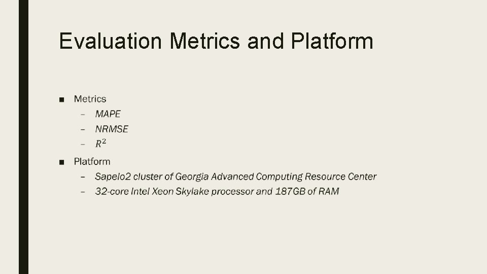
Evaluation Metrics and Platform ■

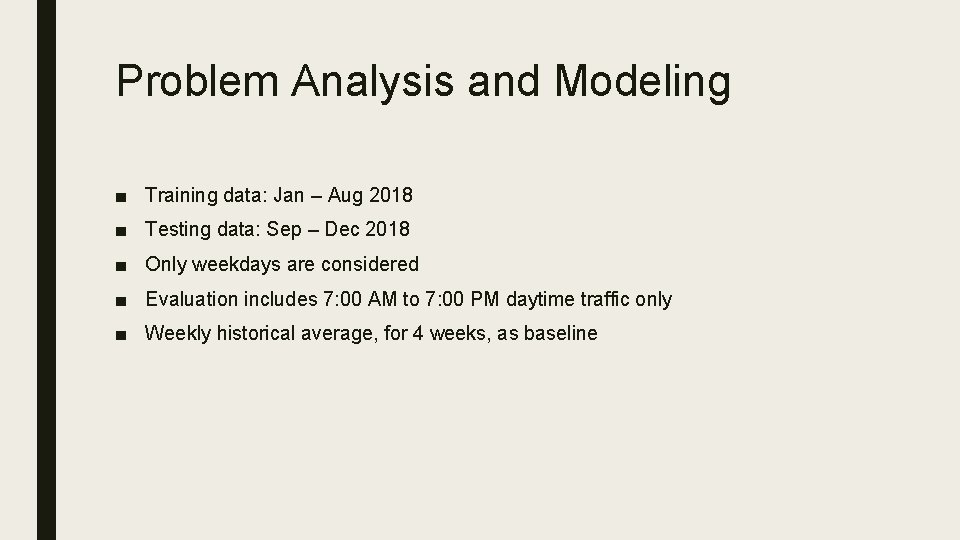
Problem Analysis and Modeling ■ Training data: Jan – Aug 2018 ■ Testing data: Sep – Dec 2018 ■ Only weekdays are considered ■ Evaluation includes 7: 00 AM to 7: 00 PM daytime traffic only ■ Weekly historical average, for 4 weeks, as baseline

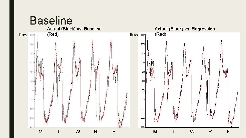
Baseline Actual (Black) vs. Baseline (Red) flow M T W R flow F Actual (Black) vs. Regression (Red) M T W R F

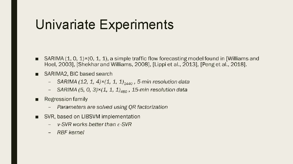
Univariate Experiments ■

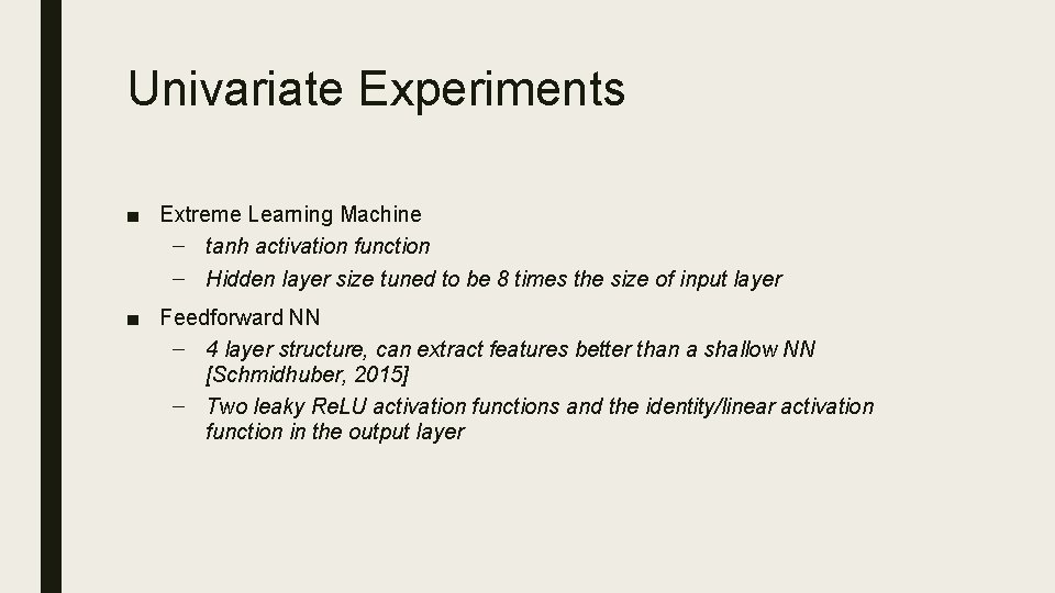
Univariate Experiments ■ Extreme Learning Machine – tanh activation function – Hidden layer size tuned to be 8 times the size of input layer ■ Feedforward NN – 4 layer structure, can extract features better than a shallow NN [Schmidhuber, 2015] – Two leaky Re. LU activation functions and the identity/linear activation function in the output layer

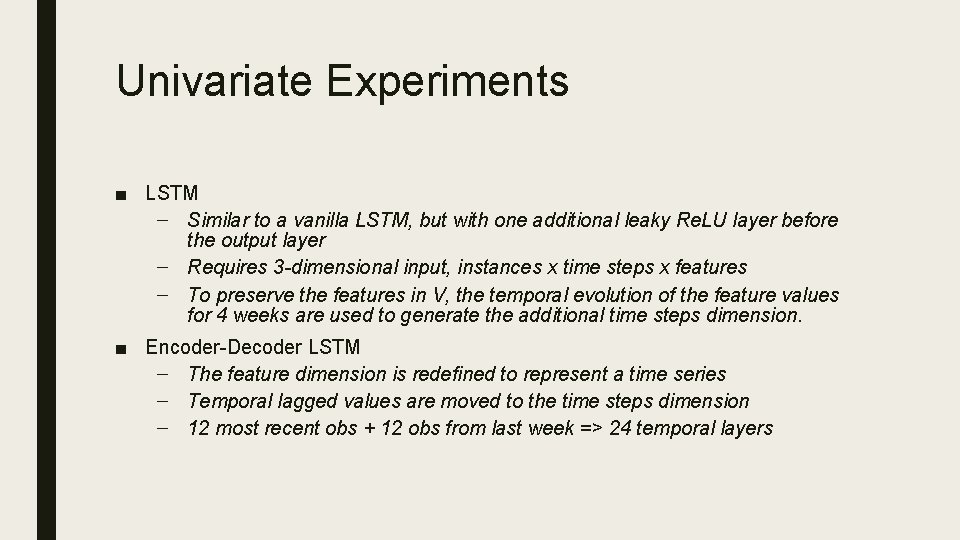
Univariate Experiments ■ LSTM – Similar to a vanilla LSTM, but with one additional leaky Re. LU layer before the output layer – Requires 3 -dimensional input, instances x time steps x features – To preserve the features in V, the temporal evolution of the feature values for 4 weeks are used to generate the additional time steps dimension. ■ Encoder-Decoder LSTM – The feature dimension is redefined to represent a time series – Temporal lagged values are moved to the time steps dimension – 12 most recent obs + 12 obs from last week => 24 temporal layers

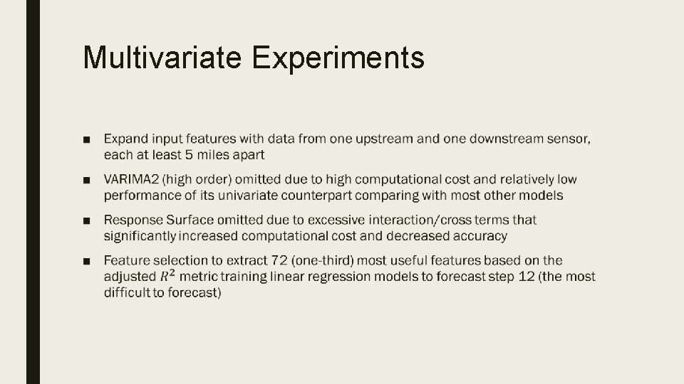
Multivariate Experiments ■

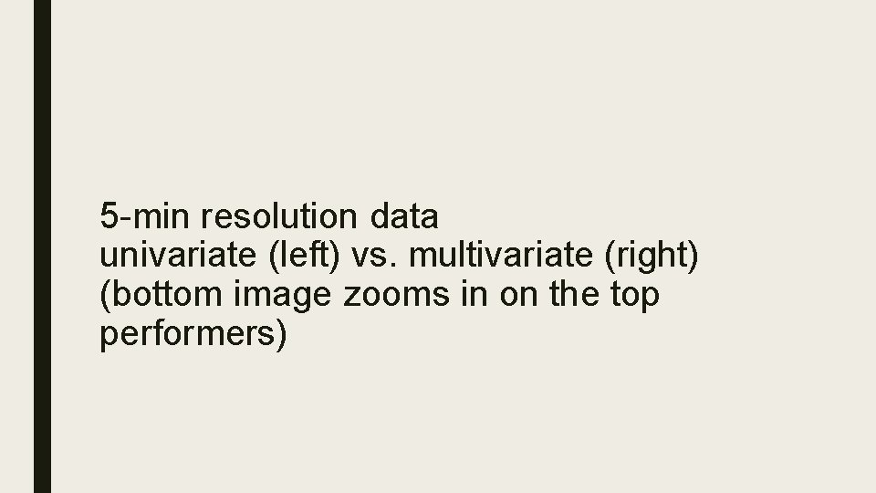
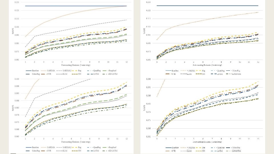
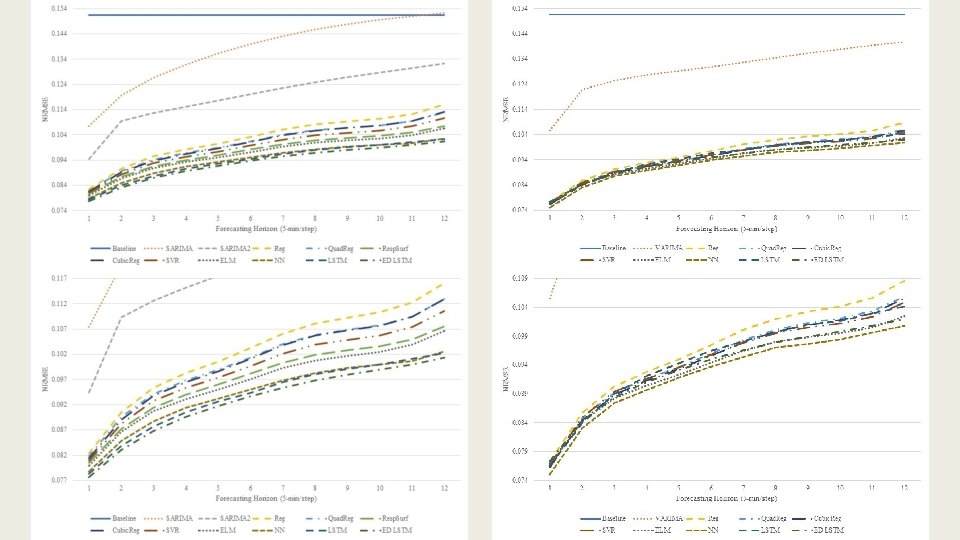
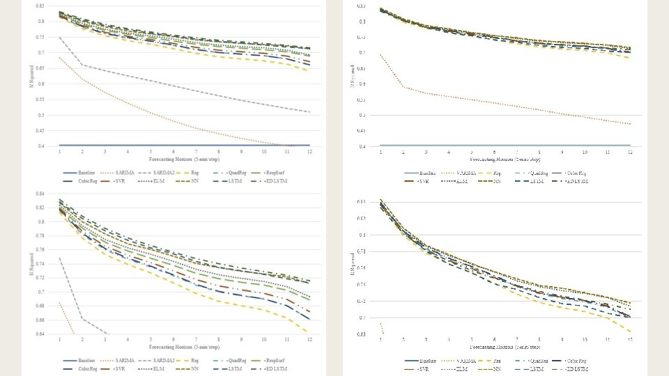
5 -min resolution data univariate (left) vs. multivariate (right) (bottom image zooms in on the top performers)

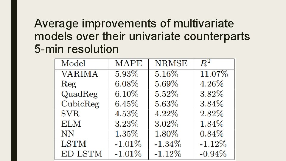
Average improvements of multivariate models over their univariate counterparts 5 -min resolution

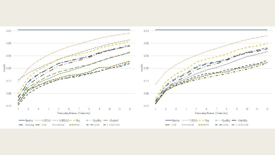
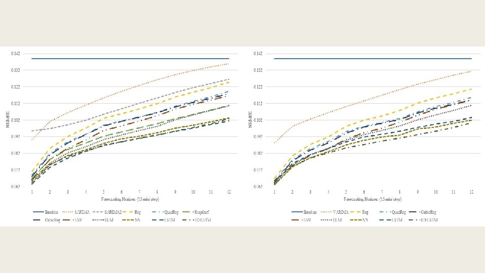
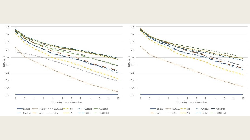
15 -min resolution data univariate (left) vs. multivariate (right)

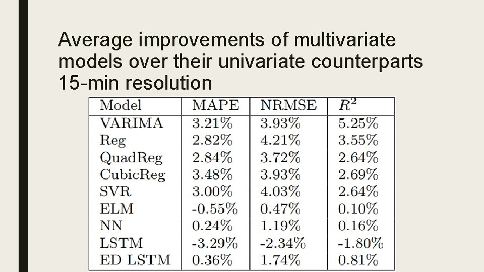
Average improvements of multivariate models over their univariate counterparts 15 -min resolution

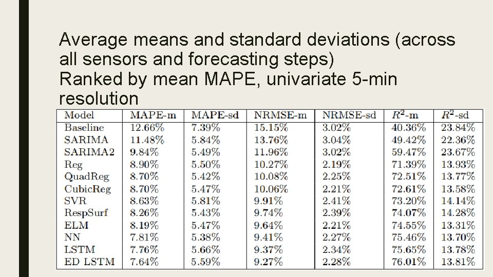
Average means and standard deviations (across all sensors and forecasting steps) Ranked by mean MAPE, univariate 5 -min resolution

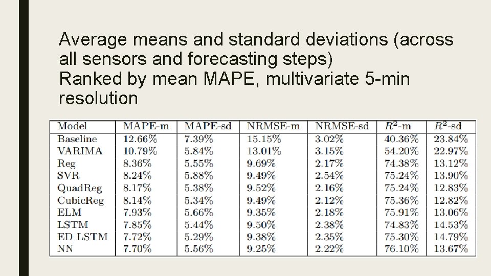
Average means and standard deviations (across all sensors and forecasting steps) Ranked by mean MAPE, multivariate 5 -min resolution

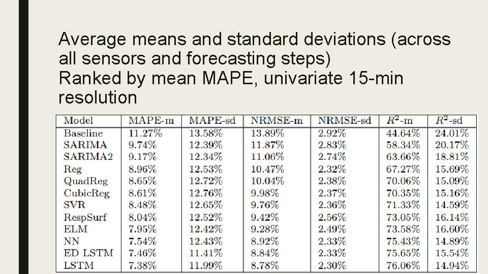
Average means and standard deviations (across all sensors and forecasting steps) Ranked by mean MAPE, univariate 15 -min resolution

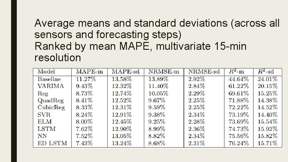
Average means and standard deviations (across all sensors and forecasting steps) Ranked by mean MAPE, multivariate 15 -min resolution

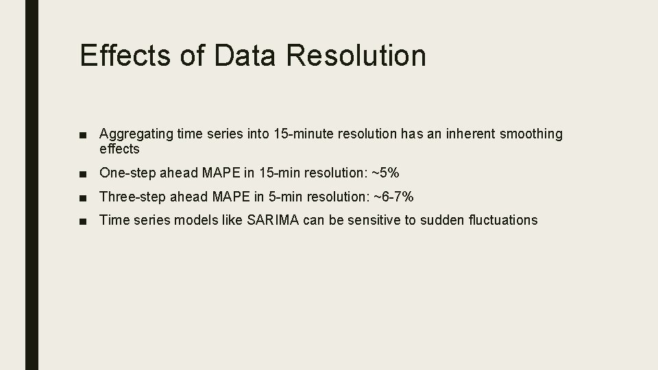
Effects of Data Resolution ■ Aggregating time series into 15 -minute resolution has an inherent smoothing effects ■ One-step ahead MAPE in 15 -min resolution: ~5% ■ Three-step ahead MAPE in 5 -min resolution: ~6 -7% ■ Time series models like SARIMA can be sensitive to sudden fluctuations

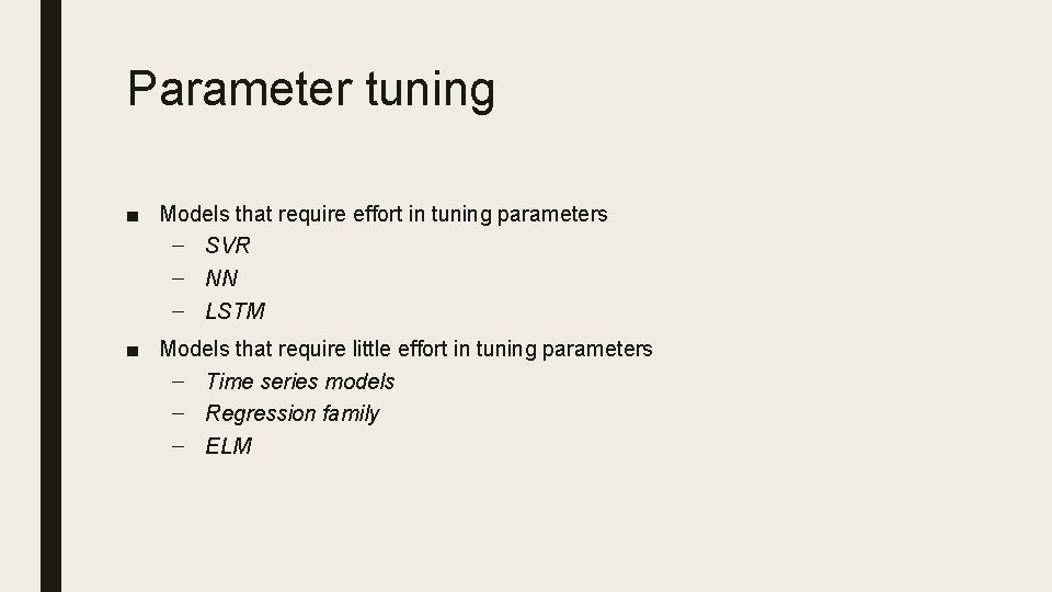
Parameter tuning ■ Models that require effort in tuning parameters – SVR – NN – LSTM ■ Models that require little effort in tuning parameters – Time series models – Regression family – ELM

Overfitting ■ NN: slight improvements in multivariate experiment ■ LSTM: minor decrease in accuracy in multivariate experiment, seems to suggest that data for the past 4 weeks may be a bit “excessive”, and causing models to unnecessarily overfitted to the traffic patterns that may not be current/useful for the immediate short terms. ■ ED LSTM: minor decrease in 5 -min multivariate experiment, minor improvements in 15 -minute multivariate experiment. It’s possible that it is easier for ED LSTM to fit the smoother 15 -minute resolution data, especially since it has 24 temporal layers. The 5 -minute resolution data are subject to more sudden fluctuations, and causing the model to be more distracted by such fluctuations. ■ All 3 keras+tensorflow neural networks use random 20% validation sets during training

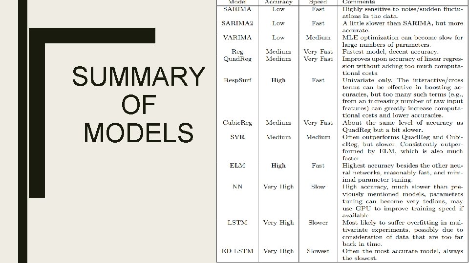
SUMMARY OF MODELS

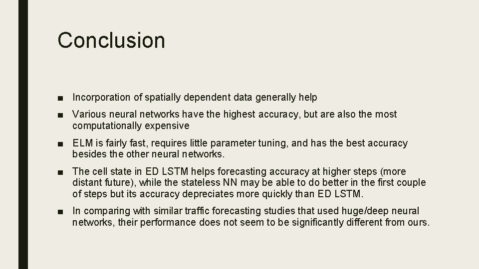
Conclusion ■ Incorporation of spatially dependent data generally help ■ Various neural networks have the highest accuracy, but are also the most computationally expensive ■ ELM is fairly fast, requires little parameter tuning, and has the best accuracy besides the other neural networks. ■ The cell state in ED LSTM helps forecasting accuracy at higher steps (more distant future), while the stateless NN may be able to do better in the first couple of steps but its accuracy depreciates more quickly than ED LSTM. ■ In comparing with similar traffic forecasting studies that used huge/deep neural networks, their performance does not seem to be significantly different from ours.

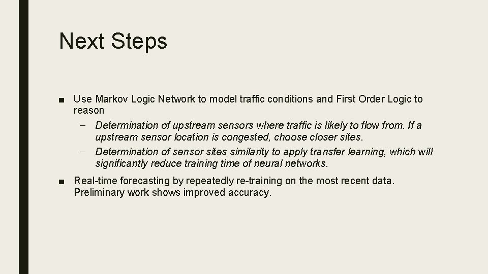
Next Steps ■ Use Markov Logic Network to model traffic conditions and First Order Logic to reason – Determination of upstream sensors where traffic is likely to flow from. If a upstream sensor location is congested, choose closer sites. – Determination of sensor sites similarity to apply transfer learning, which will significantly reduce training time of neural networks. ■ Real-time forecasting by repeatedly re-training on the most recent data. Preliminary work shows improved accuracy.

Questions?