Traditional Statistical Methods to Machine Learning Methods for

Traditional Statistical Methods to Machine Learning: Methods for Learning from Data UNC Collaborative Core Center for Clinical Research Speaker Series August 14, 2020 Jamie E. Collins, Ph. D Orthopa edic a nd Arthr itis C enter f or Outco mes Research, Brigham and Wom en’s Hospit al Department of Ort hopaedic S urgery, Harvard Medical School

Outline • Overview, Terminology • Machine Learning vs. Traditional Statistical Modeling • Examples: Statistical Modeling to Machine Learning

Overview • What is the difference between machine learning and statistical modeling? ◦ “The short answer is: None. They are both concerned with the same question: how do we learn from data? ” – Dr. Larry Wasserman, Professor of Statistics and Data Science in the Department of Statistics and Data Science and in the Machine Learning Department at Carnegie Melon https: //normaldeviate. wordpress. com/2012/06/12/statistics-versus-machine-learning-5 -2/

Overview • Machine Learning ◦ Is a method of data analysis that automates analytical model building. ◦ The process of teaching a computer system how to make accurate predictions when fed data. ◦ Gives computers the capability to learn without being explicitly programmed.

Overview • Machine Learning includes ◦ Supervised Methods ◦ Unsupervised Methods ◦ Semi-Supervised Methods

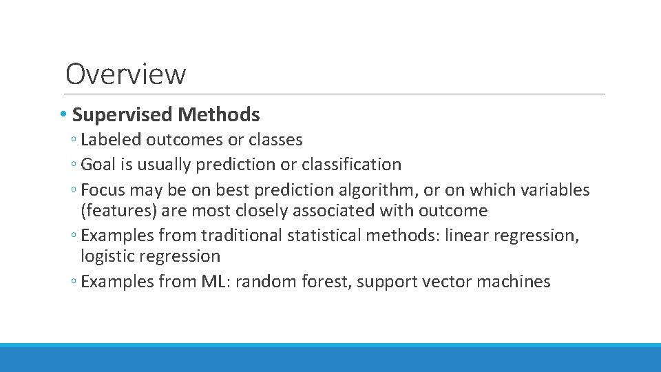
Overview • Supervised Methods ◦ Labeled outcomes or classes ◦ Goal is usually prediction or classification ◦ Focus may be on best prediction algorithm, or on which variables (features) are most closely associated with outcome ◦ Examples from traditional statistical methods: linear regression, logistic regression ◦ Examples from ML: random forest, support vector machines

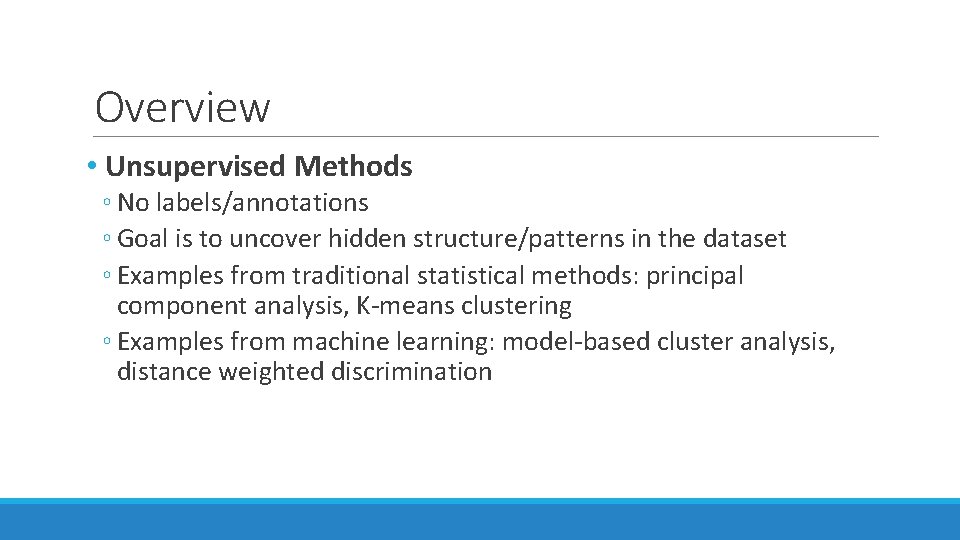
Overview • Unsupervised Methods ◦ No labels/annotations ◦ Goal is to uncover hidden structure/patterns in the dataset ◦ Examples from traditional statistical methods: principal component analysis, K-means clustering ◦ Examples from machine learning: model-based cluster analysis, distance weighted discrimination

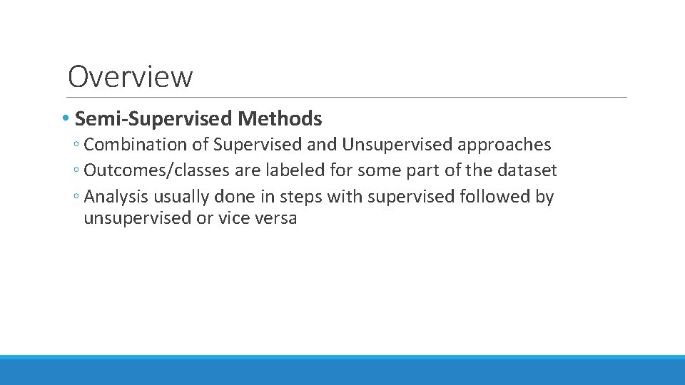
Overview • Semi-Supervised Methods ◦ Combination of Supervised and Unsupervised approaches ◦ Outcomes/classes are labeled for some part of the dataset ◦ Analysis usually done in steps with supervised followed by unsupervised or vice versa

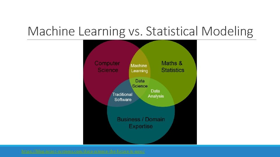
Machine Learning vs. Statistical Modeling https: //blog. intact-systems. com/data-science-the-future-is-now/

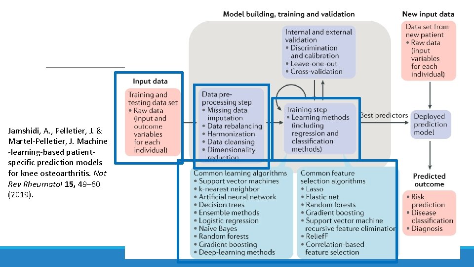
Jamshidi, A. , Pelletier, J. & Martel-Pelletier, J. Machine -learning-based patientspecific prediction models for knee osteoarthritis. Nat Rev Rheumatol 15, 49– 60 (2019).

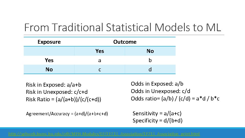
From Traditional Statistical Models to ML Exposure Yes No Outcome Yes a c Risk in Exposed: a/a+b Risk in Unexposed: c/c+d Risk Ratio = (a/(a+b))/(c/(c+d)) Agreement/Accuracy = (a+d)/(a+b+c+d) No b d Odds in Exposed: a/b Odds in Unexposed: c/d Odds ratio= (a/b) / (c/d) = a*d / b*c Sensitivity = a/(a+c) Specificity = d/(b+d) http: //sphweb. bumc. bu. edu/otlt/MPH-Modules/EP/EP 713_Association_print. html

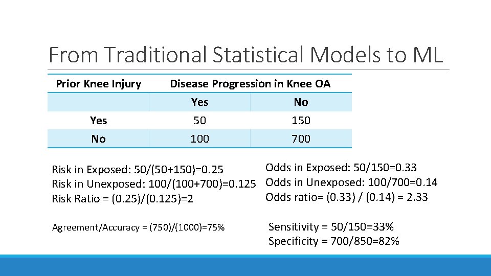
From Traditional Statistical Models to ML Prior Knee Injury Yes No Disease Progression in Knee OA Yes No 50 100 700 Odds in Exposed: 50/150=0. 33 Risk in Exposed: 50/(50+150)=0. 25 Risk in Unexposed: 100/(100+700)=0. 125 Odds in Unexposed: 100/700=0. 14 Odds ratio= (0. 33) / (0. 14) = 2. 33 Risk Ratio = (0. 25)/(0. 125)=2 Agreement/Accuracy = (750)/(1000)=75% Sensitivity = 50/150=33% Specificity = 700/850=82%

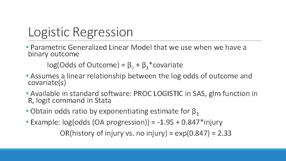
Logistic Regression • Parametric Generalized Linear Model that we use when we have a binary outcome log(Odds of Outcome) = β 0 + β 1*covariate • Assumes a linear relationship between the log odds of outcome and covariate(s) • Available in standard software: PROC LOGISTIC in SAS, glm function in R, logit command in Stata • Obtain odds ratio by exponentiating estimate for β 1 • Example: log(odds (OA progression)) = -1. 95 + 0. 847*injury OR(history of injury vs. no injury) = exp(0. 847) = 2. 33

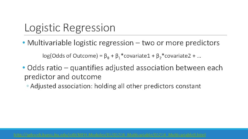
Logistic Regression • Multivariable logistic regression – two or more predictors log(Odds of Outcome) = β 0 + β 1*covariate 1 + β 2*covariate 2 + … • Odds ratio – quantifies adjusted association between each predictor and outcome ◦ Adjusted association: holding all other predictors constant http: //sphweb. bumc. bu. edu/otlt/MPH-Modules/BS/BS 704_Multivariable 8. html

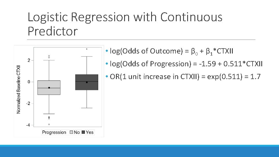
Logistic Regression with Continuous Predictor • log(Odds of Outcome) = β 0 + β 1*CTXII • log(Odds of Progression) = -1. 59 + 0. 511*CTXII • OR(1 unit increase in CTXII) = exp(0. 511) = 1. 7

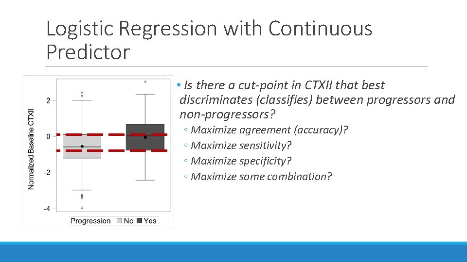
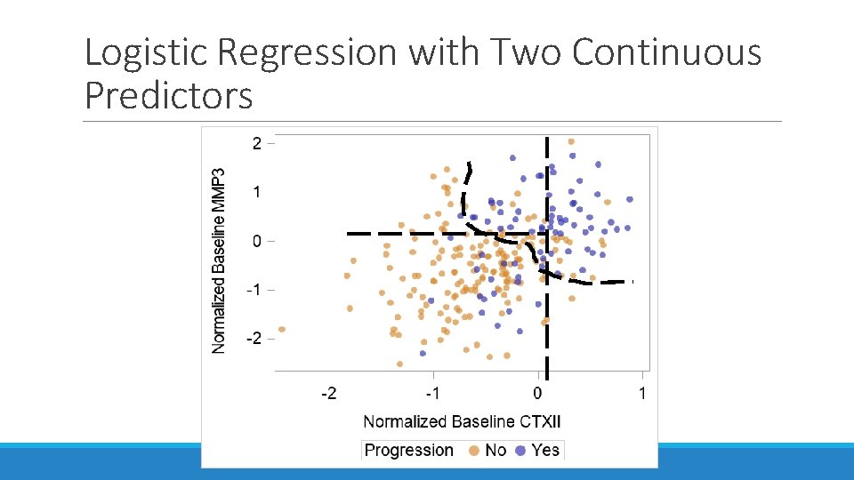
Logistic Regression with Continuous Predictor • Is there a cut-point in CTXII that best discriminates (classifies) between progressors and non-progressors? ◦ Maximize agreement (accuracy)? ◦ Maximize sensitivity? ◦ Maximize specificity? ◦ Maximize some combination?

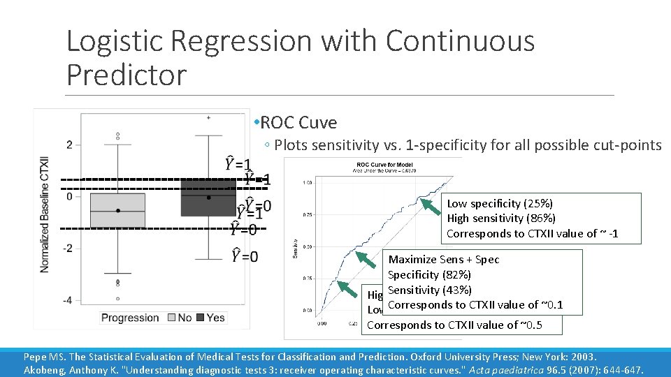
Logistic Regression with Continuous Predictor • ROC Cuve ◦ Plots sensitivity vs. 1 -specificity for all possible cut-points Low specificity (25%) High sensitivity (86%) Corresponds to CTXII value of ~ -1 Maximize Sens + Specificity (82%) High. Sensitivity specificity(43%) (87. 5%) to CTXII value of ~0. 1 Low. Corresponds sensitivity (26%) Corresponds to CTXII value of ~0. 5 Pepe MS. The Statistical Evaluation of Medical Tests for Classification and Prediction. Oxford University Press; New York: 2003. Akobeng, Anthony K. "Understanding diagnostic tests 3: receiver operating characteristic curves. " Acta paediatrica 96. 5 (2007): 644 -647.

Logistic Regression with Two Continuous Predictors

Logistic Regression • Sample Size – rule of thumb: 10 outcomes for each predictor (really, each degree of freedom) ◦ E. g. , in our OA progression example, n=1000 ◦ n=250 progressors ◦ n=750 non-progressors ◦ Suggests model with ~25 predictors • How do we choose the “best” combination of predictors? • What if the number of predictors > 25? • What if the number of predictors > 1000? (p>n) • Overfitting: the model should generalize to populations that were not included in the sample. Overfitting is when the model captures random variation in the data.

Regression Selection Procedures • Backward ◦ Start with all predictors in the model, remove the predictor with the highest pvalue, continue until all p-values are < p-critical (e. g. , 0. 05). • Forward ◦ Start with predictor with lowest p-value (and < p-critical), check each remaining predictor to find adjusted p-value and add predictor with smallest p-value. Continue until no more predictors reach p < p-critical. • Stepwise ◦ Combines backward and forward. Start as in forward with predictor with lowest pvalue, add predictor with lowest adjusted p-value. Now go back, and check original predictor, if p > p-crit for this predictor, then remove. After each new predictor is added, go back and check every other predictor in the model. * Can also do this based on other fit statistics (e. g. , AIC, BIC, adjusted R 2) Steyerberg, Ewout W. Clinical prediction models. Springer International Publishing, 2019. Hosmer DW, Lemeshow S: Applied Logistic Regression. 2000, New York: Wiley

Regression Selection Procedures • Best Subsets ◦ Check every possible subset of variables, and choose the subset with the best fit (e. g. , based on set criteria like AIC, BIC, R 2) Steyerberg, Ewout W. Clinical prediction models. Springer International Publishing, 2019. Hosmer DW, Lemeshow S: Applied Logistic Regression. 2000, New York: Wiley

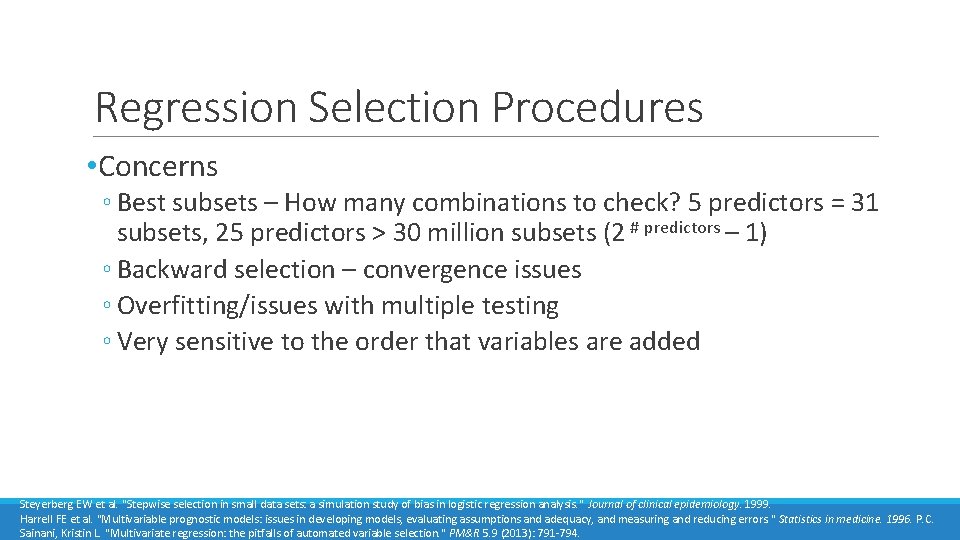
Regression Selection Procedures • Concerns ◦ Best subsets – How many combinations to check? 5 predictors = 31 subsets, 25 predictors > 30 million subsets (2 # predictors – 1) ◦ Backward selection – convergence issues ◦ Overfitting/issues with multiple testing ◦ Very sensitive to the order that variables are added Steyerberg EW et al. "Stepwise selection in small data sets: a simulation study of bias in logistic regression analysis. " Journal of clinical epidemiology. 1999. Harrell FE et al. "Multivariable prognostic models: issues in developing models, evaluating assumptions and adequacy, and measuring and reducing errors. " Statistics in medicine. 1996. P. C. Sainani, Kristin L. "Multivariate regression: the pitfalls of automated variable selection. " PM&R 5. 9 (2013): 791 -794.

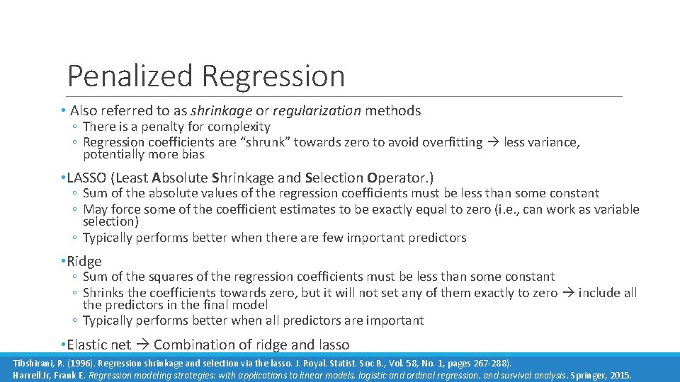
Penalized Regression • Also referred to as shrinkage or regularization methods ◦ There is a penalty for complexity ◦ Regression coefficients are “shrunk” towards zero to avoid overfitting less variance, potentially more bias • LASSO (Least Absolute Shrinkage and Selection Operator. ) ◦ Sum of the absolute values of the regression coefficients must be less than some constant ◦ May force some of the coefficient estimates to be exactly equal to zero (i. e. , can work as variable selection) ◦ Typically performs better when there are few important predictors • Ridge ◦ Sum of the squares of the regression coefficients must be less than some constant ◦ Shrinks the coefficients towards zero, but it will not set any of them exactly to zero include all the predictors in the final model ◦ Typically performs better when all predictors are important • Elastic net Combination of ridge and lasso Tibshirani, R. (1996). Regression shrinkage and selection via the lasso. J. Royal. Statist. Soc B. , Vol. 58, No. 1, pages 267 -288). Harrell Jr, Frank E. Regression modeling strategies: with applications to linear models, logistic and ordinal regression, and survival analysis. Springer, 2015.

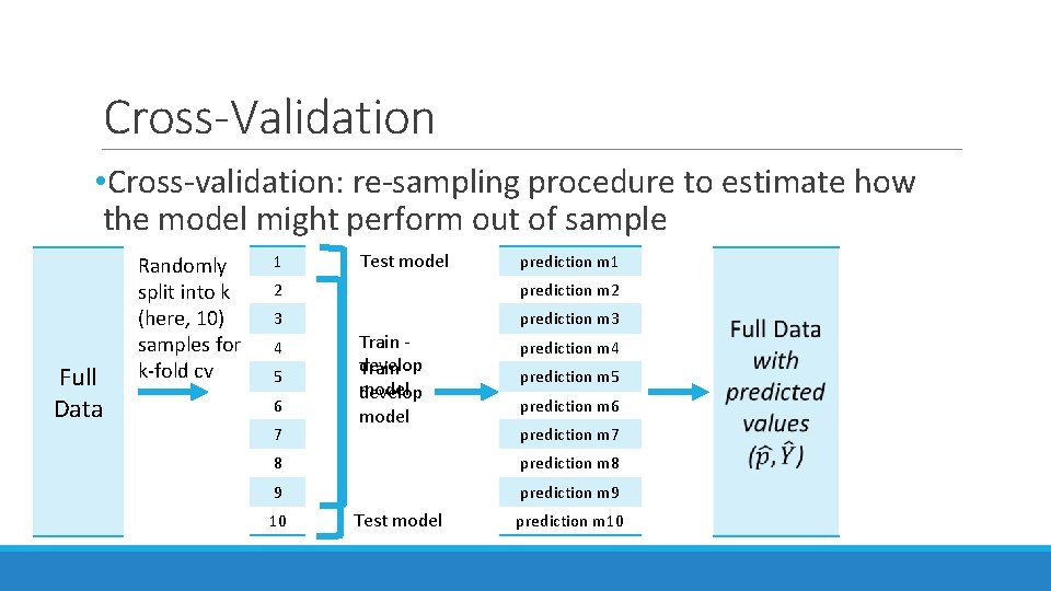
Cross-Validation • Cross-validation: re-sampling procedure to estimate how the model might perform out of sample Full Data Randomly split into k (here, 10) samples for k-fold cv 1 Test model prediction m 1 2 prediction m 2 3 prediction m 3 4 5 6 7 Train develop Train model develop model prediction m 4 prediction m 5 prediction m 6 prediction m 7 8 prediction m 8 9 prediction m 9 10 Test model prediction m 10

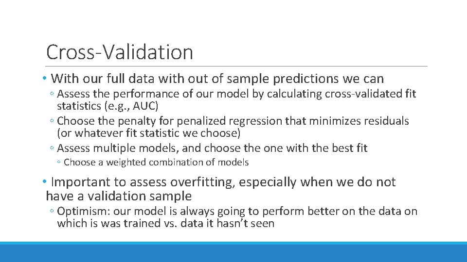
Cross-Validation • With our full data with out of sample predictions we can ◦ Assess the performance of our model by calculating cross-validated fit statistics (e. g. , AUC) ◦ Choose the penalty for penalized regression that minimizes residuals (or whatever fit statistic we choose) ◦ Assess multiple models, and choose the one with the best fit ◦ Choose a weighted combination of models • Important to assess overfitting, especially when we do not have a validation sample ◦ Optimism: our model is always going to perform better on the data on which is was trained vs. data it hasn’t seen

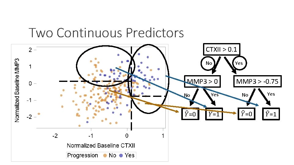
Two Continuous Predictors CTXII > 0. 1 No MMP 3 > 0 No Yes MMP 3 > -0. 75 No Yes

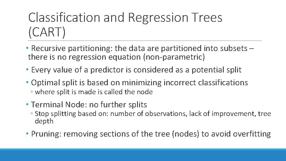
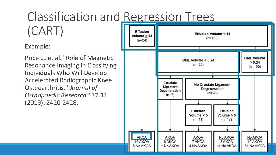
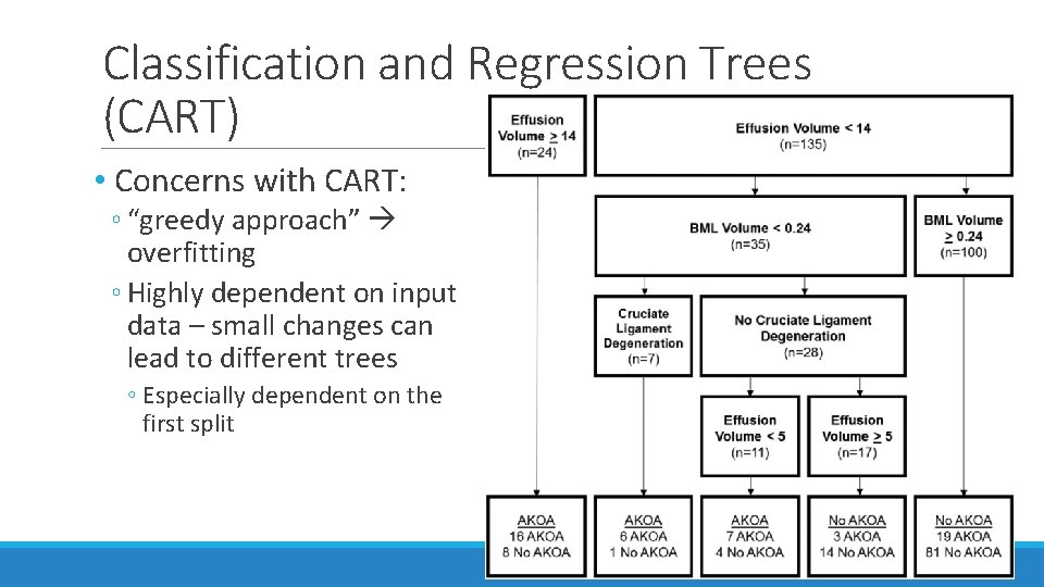
Classification and Regression Trees (CART) • Recursive partitioning: the data are partitioned into subsets – there is no regression equation (non-parametric) • Every value of a predictor is considered as a potential split • Optimal split is based on minimizing incorrect classifications ◦ where split is made is called the node • Terminal Node: no further splits ◦ Stop splitting based on: number of observations, lack of improvement, tree depth • Pruning: removing sections of the tree (nodes) to avoid overfitting

Classification and Regression Trees (CART) Example: Price LL et al. "Role of Magnetic Resonance Imaging in Classifying Individuals Who Will Develop Accelerated Radiographic Knee Osteoarthritis. " Journal of Orthopaedic Research® 37. 11 (2019): 2420 -2428.

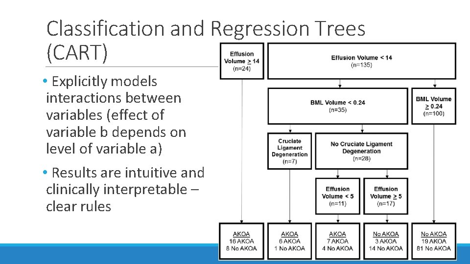
Classification and Regression Trees (CART) • Explicitly models interactions between variables (effect of variable b depends on level of variable a) • Results are intuitive and clinically interpretable – clear rules

Classification and Regression Trees (CART) • Concerns with CART: ◦ “greedy approach” overfitting ◦ Highly dependent on input data – small changes can lead to different trees ◦ Especially dependent on the first split

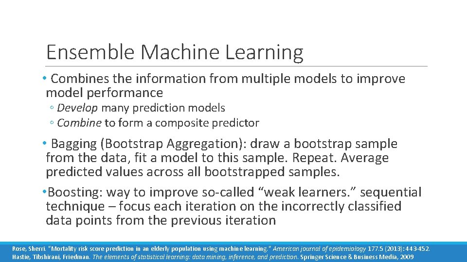
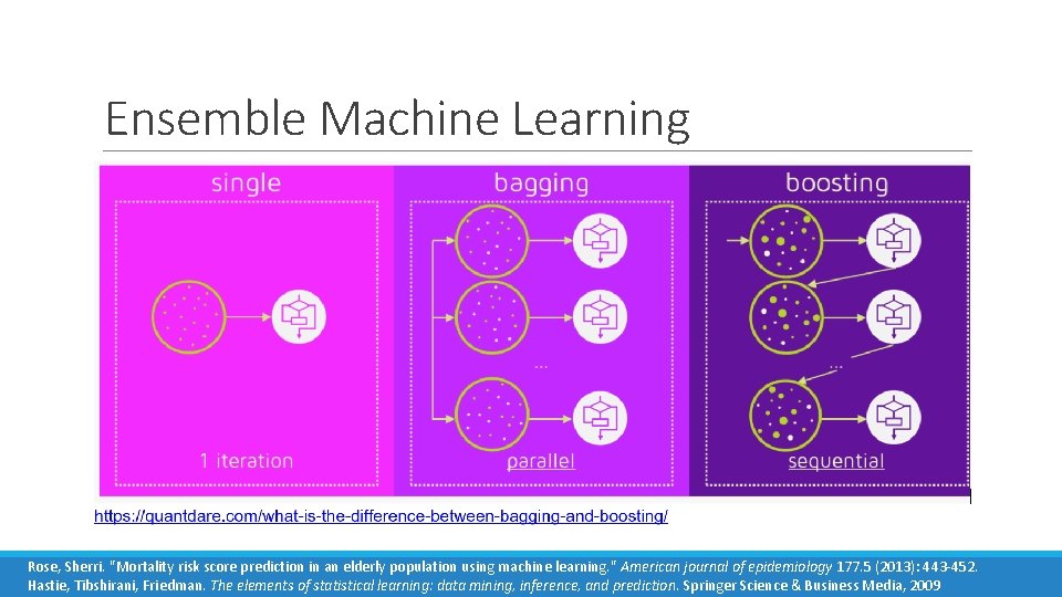
Ensemble Machine Learning • Combines the information from multiple models to improve model performance ◦ Develop many prediction models ◦ Combine to form a composite predictor • Bagging (Bootstrap Aggregation): draw a bootstrap sample from the data, fit a model to this sample. Repeat. Average predicted values across all bootstrapped samples. • Boosting: way to improve so-called “weak learners. ” sequential technique – focus each iteration on the incorrectly classified data points from the previous iteration Rose, Sherri. "Mortality risk score prediction in an elderly population using machine learning. " American journal of epidemiology 177. 5 (2013): 443 -452. Hastie, Tibshirani, Friedman. The elements of statistical learning: data mining, inference, and prediction. Springer Science & Business Media, 2009

Ensemble Machine Learning • Combines the information from multiple models to improve model performance • Develop many prediction models • Combine to form a composite predictor • Bagging (Bootstrap Aggregation): draw a bootstrap sample from the data, fit a model to this sample. Repeat. Average predicted values across all bootstrapped samples. • Boosting: way to improve so-called “weak learners. ” sequential technique – focus each iteration on incorrectly classified data points from the previous iteration Rose, Sherri. "Mortality risk score prediction in an elderly population using machine learning. " American journal of epidemiology 177. 5 (2013): 443 -452. Hastie, Tibshirani, Friedman. The elements of statistical learning: data mining, inference, and prediction. Springer Science & Business Media, 2009

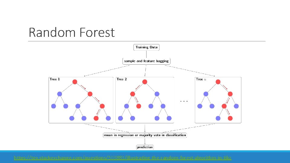
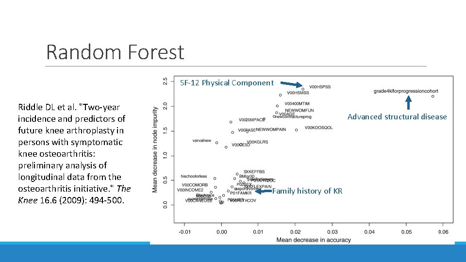
Random Forest • Tree-based approach (like CART) with bagging • Draw a random sample of subjects and a random sample of predictors and then create decision tree • Average across trees • Pros: improved prediction, more stable • Cons: interpretability – we can use measures to assess variable importance, but there is no clear measure to assess the association between predictors and outcome (e. g. , OR), no final tree

Random Forest https: //tex. stackexchange. com/questions/503883/illustrating-the-random-forest-algorithm-in-tikz

Random Forest SF-12 Physical Component Riddle DL et al. "Two-year incidence and predictors of future knee arthroplasty in persons with symptomatic knee osteoarthritis: preliminary analysis of longitudinal data from the osteoarthritis initiative. " The Knee 16. 6 (2009): 494 -500. Advanced structural disease Family history of KR

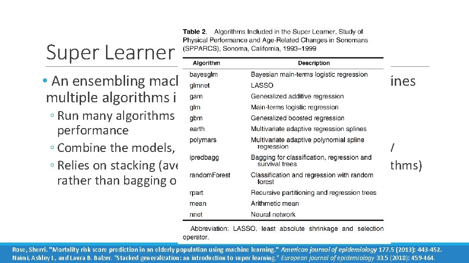
Super Learner • An ensembling machine learning approach that combines multiple algorithms into a single algorithm. ◦ Run many algorithms – use cross-validation to assess model performance ◦ Combine the models, weighting by model performance in CV ◦ Relies on stacking (averaging across multiple different algorithms) rather than bagging or boosting Rose, Sherri. "Mortality risk score prediction in an elderly population using machine learning. " American journal of epidemiology 177. 5 (2013): 443 -452. Naimi, Ashley I. , and Laura B. Balzer. "Stacked generalization: an introduction to super learning. " European journal of epidemiology 33. 5 (2018): 459 -464.

Super Learner • An ensembling machine learning approach that combines multiple algorithms into a single algorithm. ◦ Run many algorithms – use cross-validation to assess model performance ◦ Combine the models, weighting by model performance in CV ◦ Relies on stacking (averaging across multiple different algorithms) rather than bagging or boosting Rose, Sherri. "Mortality risk score prediction in an elderly population using machine learning. " American journal of epidemiology 177. 5 (2013): 443 -452. Naimi, Ashley I. , and Laura B. Balzer. "Stacked generalization: an introduction to super learning. " European journal of epidemiology 33. 5 (2018): 459 -464.

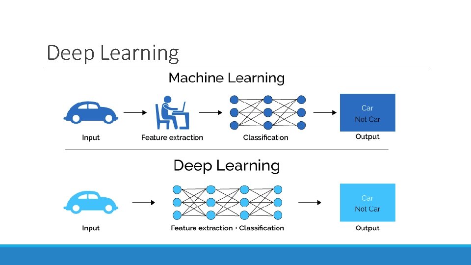
Deep Learning

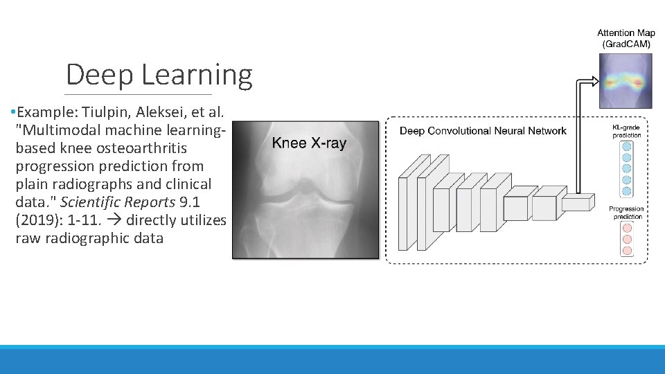
Deep Learning • Example: Tiulpin, Aleksei, et al. "Multimodal machine learningbased knee osteoarthritis progression prediction from plain radiographs and clinical data. " Scientific Reports 9. 1 (2019): 1 -11. directly utilizes raw radiographic data

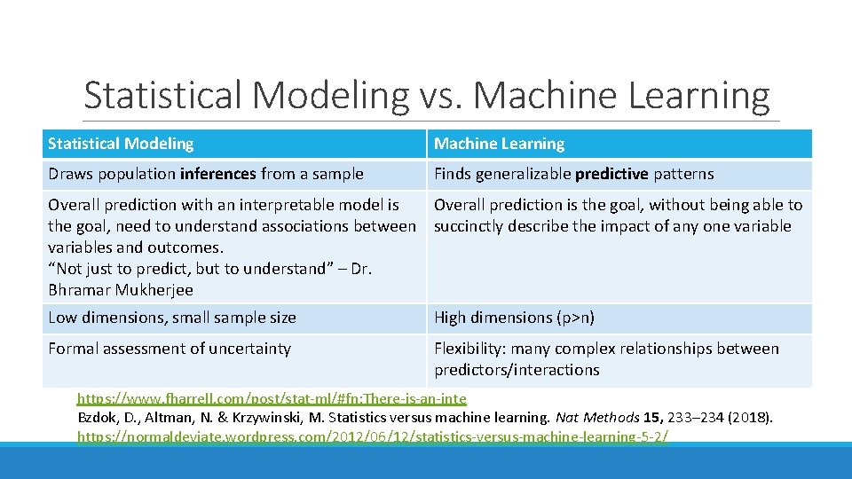
Statistical Modeling vs. Machine Learning Statistical Modeling Machine Learning Draws population inferences from a sample Finds generalizable predictive patterns Overall prediction with an interpretable model is Overall prediction is the goal, without being able to the goal, need to understand associations between succinctly describe the impact of any one variables and outcomes. “Not just to predict, but to understand” – Dr. Bhramar Mukherjee Low dimensions, small sample size High dimensions (p>n) Formal assessment of uncertainty Flexibility: many complex relationships between predictors/interactions https: //www. fharrell. com/post/stat-ml/#fn: There-is-an-inte Bzdok, D. , Altman, N. & Krzywinski, M. Statistics versus machine learning. Nat Methods 15, 233– 234 (2018). https: //normaldeviate. wordpress. com/2012/06/12/statistics-versus-machine-learning-5 -2/

References • Hastie, Tibshirani, Friedman. The elements of statistical learning: data mining, inference, and prediction. Springer Science & Business Media, 2009. • Harrell Jr, Frank E. Regression modeling strategies: with applications to linear models, logistic and ordinal regression, and survival analysis. Springer, 2015. • Pepe MS. The Statistical Evaluation of Medical Tests for Classification and Prediction. Oxford University Press; New York: 2003. • Steyerberg, Ewout W. Clinical prediction models. Springer International Publishing, 2019. • van der Laan MJ, Rose S. Targeted Learning: Causal Inference for Observational and Experimental Data. Springer, 2011. • Collins, Gary S. , et al. "Transparent Reporting of a Multivariable Prediction Model for Individual Prognosis or Diagnosis (TRIPOD) The TRIPOD Statement. " Circulation 131. 2 (2015): 211 -219.

References • Maria Hügle, Patrick Omoumi, Jacob M van Laar, Joschka Boedecker, Thomas Hügle, Applied machine learning and artificial intelligence in rheumatology, Rheumatology Advances in Practice, Volume 4, Issue 1, 2020 • Bzdok, D. , Altman, N. & Krzywinski, M. Statistics versus machine learning. Nat Methods 15, 233– 234 (2018). • Jamshidi, A. , Pelletier, J. & Martel-Pelletier, J. Machine-learning-based patient-specific prediction models for knee osteoarthritis. Nat Rev Rheumatol 15, 49– 60 (2019). • Sherri Rose, Intersections of machine learning and epidemiological methods for health services research, International Journal of Epidemiology, , dyaa 035, https: //doi. org/10. 1093/ije/dyaa 035

Thank You! JCollins 13@bwh. harvard. edu @Coll. Jamie