Traditional Keynesian Theories of Fluctuations From Romer chapter
")

 • Time")


 are CRRA The assumption that Money enter the utility")


 is added to the traditional IS curve With uncertainty, we")


 LM(P 1) The aggregate demand curve IS Y P P 0")
 IS(G 1) IS(G 0) Y P AS AS AD 1 AD")
 i LM(P 1) IS Yn Y")

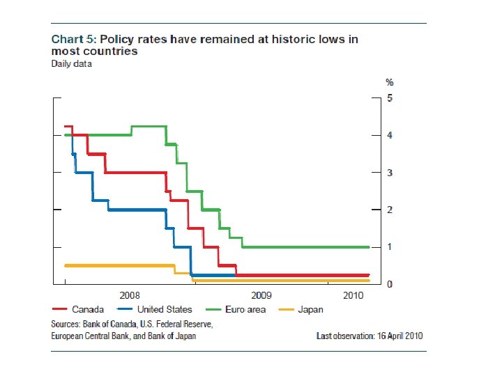
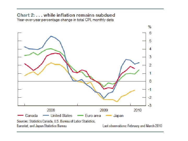
 Monetary Policy in Deflation: The Liquidity Trap")
 Monetary Policy in Deflation: The Liq in History and Practice.")


 L")


- Slides: 27
Traditional Keynesian Theories of Fluctuations (From Romer, chapter 6 part A, section 7. 8) • • Microfundations The IS-LM-AD model The liquidity trap and the post 2008 crisis The supply curve The open economy and exchange rate overshooting The Phillips curve The natural rate of unemployment The Canonical New-Keynesian model • Introduction
Structure of a Keynesian model • Aggregate demand – IS curve (flow equilibrium: the Keynesian cross) – LM curve (stock equilibrium, financial market, money market) • Aggregate supply P AS – Labour market – Production function AD Y AS curve not vertical
IS-LM model with fixed prices • Nominal rigidities are given (fixed prices) • Time is discrete capital is fixed, closed economy, no government to start with • The production function is:
Household optimization problem • Fixed number of infinitely lived households • They get utility from consumption, holding money, and disutility from working • We ignore population growth and normalize the number of household to 1
Household objective function is
Utility functions (C and M) are CRRA The assumption that Money enter the utility function is a short cut Observationally equivalent to transaction purpose (Fenstra 1986)
Money and Bonds: Two assets • The two assets are substitute • Bonds bears interest rate but are not liquid (i. e. , in the U function)
• For households, paths of P, W, and I are given • Path of C and M are chosen in order to maximize 6. 2 subject to (6. 5) and the No-Ponzi game condition • For the moment, L is exogenous • Path of M is set by the central bank
New Keynesian IS curve • Following Romer intuitive methodology to derive the Euler equation (last paragraph of page 240) with the real interest rate is:
• • Y(t+1) is added to the traditional IS curve With uncertainty, we have instead E(Y(t+1) Inverse relationship between Y(t) and r(t). Relationship is strengthen with the introduction of capital and investment (chapter 9 of book)
LM curve • Again following Romer approach to optimization (bottom of page 241 do it yourself). • First order condition for money holding (an increase in m increase utility of money holding but decrease return on bond holding and consumption (6. 9)
• The LM curve in increasing in output and decreasing in the nominal interest rate (explanation) • Interest rate rule is the modern approach to close the system
i LM(P 0) LM(P 1) The aggregate demand curve IS Y P P 0 P 1 AD Y
i LM(P 0) IS(G 1) IS(G 0) Y P AS AS AD 1 AD 0 Y
The liquidity trap In this case: LM(P 0) i LM(P 1) IS Yn Y
-What is the shape of the AD curve in this case? -What happen if the AS curve is vertical (classical) -What about the Pigou effect? -This is related to Summers (1991)
Source : Orphanides (2003) Monetary Policy in Deflation: The Liquidity Trap
Source : Orphanides (2003) Monetary Policy in Deflation: The Liq in History and Practice. Miméo, FED
• • • The remedy should come, I suggest, from a general recognition that the rate of investment need not be beyond our control, if we are prepared to use our banking systems to effect a proper adjustment of the market-rate of interest. It might be sufficient merely to produce a general belief in the long continuance of a very low rate of short-term interest. The change, once it has begun, will feed on itself. . The Bank of England the Federal Reserve Board. . . should pursue bank -rate policy and open-market operations a outrance. . . [t]hat is to say, they should combine to maintain a very low level of the short-term rate of interest, and buy long-dated securities. . . until the short-term market is saturated.
The aggregate supply curve Alternative assumptions about wage and price rigidity section 5. 3 Four cases studied: 1) Rigid nominal wages (Keynes’s model) W/P 1 LS E A decrease in the price level (AD shock) A W/P 0 LD L W/P counter-cyclical rejected by facts W/P moderately pro-cyclical
P AS Y
Case 2: Sticky Prices, Flexible Wages, Competitive Labour Market AS P AD And Y is determined by AD, the effective demand for labour is determined by AD Y
W/P LD LS The effective demand for labour E Pro-cyclical real wage F-1(Y) L
W/P LD LS One reason for this is the efficiency-wage E If w flatter than LS, u↑ w(L) F-1(Y) L Case 3: Sticky Prices, Flexible wages, Real Labour Market Imperfections
Case 4: Sticky Wages, Flexible Prices, Imperfect Competition Markup function If μ is fixed, W/P counter cyclical as in case 1 However, if μ is countercyclical (strong evidences), the real wage can be acyclical or procyclical.