Tracking with Kalman Filter Based on Computer vision

Tracking with Kalman Filter Based on “Computer vision – A modern Approach” Brad C. YU The Australian National University 01 August 2005 1

Outline • • Motivation Tracking in Linear Dynamic Models The Kalman Filter (KF) KF for Nonlinear models What? Why? How? 2

What is tracking? • Tracking is the problem of generating an inference about the motion of an object given a sequence of images. • Analogies of “tracking” – – A spy “following” you A missile “targeting” a ship A detective “spotting” the suspects A typical scene of “chasing car” in a Hollywood movie 3

Surveillance Mike Isard and Andrew Blake 4

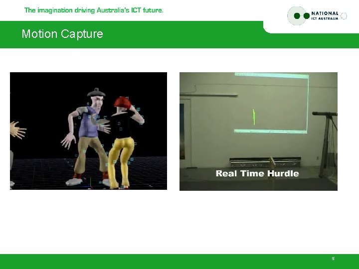
Motion Capture 5

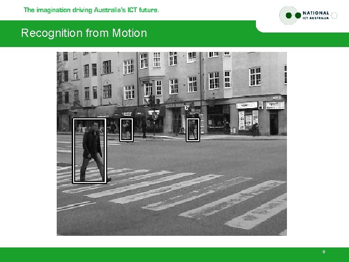
Recognition from Motion 6

Targeting 7

Why Tracking? • Motion capture • Recognition from motion • Surveillance HOW do we do it? • Targeting • Any other applications you can think of ~ 8

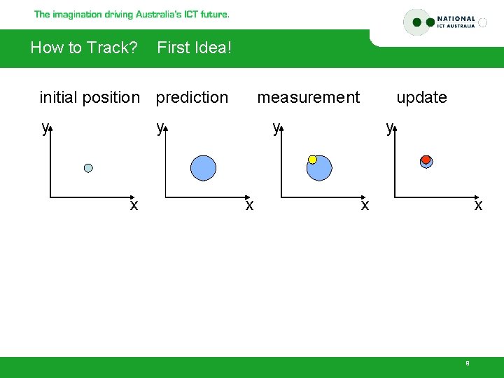
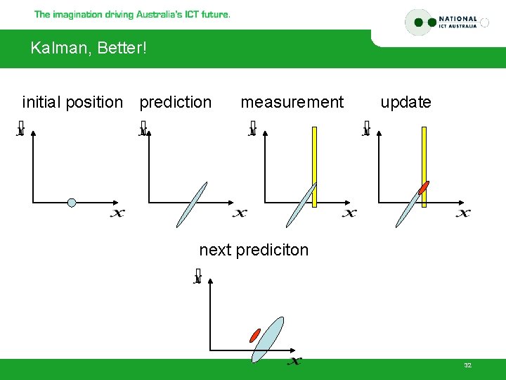
How to Track? First Idea! initial position prediction y measurement y x update y x x 9

Outline • • Motivation Tracking in Linear Dynamic Models The Kalman Filter (KF) KF for Nonlinear models 10

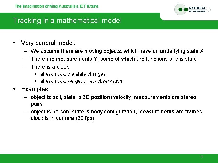
Tracking in a mathematical model • Very general model: – We assume there are moving objects, which have an underlying state X – There are measurements Y, some of which are functions of this state – There is a clock • at each tick, the state changes • at each tick, we get a new observation • Examples – object is ball, state is 3 D position+velocity, measurements are stereo pairs – object is person, state is body configuration, measurements are frames, clock is in camera (30 fps) 11

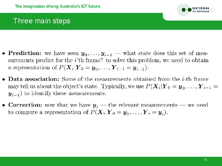
Three main steps 12

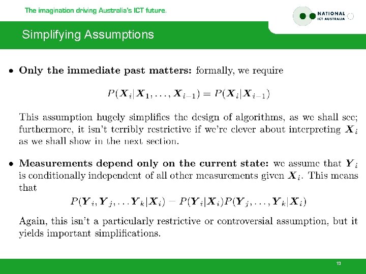
Simplifying Assumptions 13

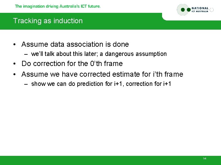
Tracking as induction • Assume data association is done – we’ll talk about this later; a dangerous assumption • Do correction for the 0’th frame • Assume we have corrected estimate for i’th frame – show we can do prediction for i+1, correction for i+1 14

Base case 15

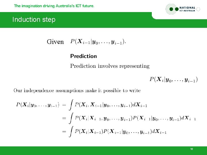
Induction step Given 16

Induction step 17

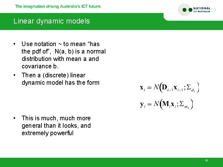
Linear dynamic models • Use notation ~ to mean “has the pdf of”, N(a, b) is a normal distribution with mean a and covariance b. • Then a (discrete) linear dynamic model has the form • This is much, much more general than it looks, and extremely powerful 18

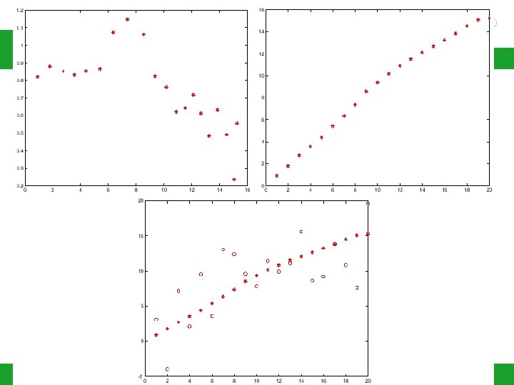
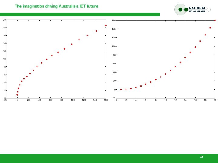
Examples • Drifting points – we assume that the new position of the point is the old one, plus noise. – For the measurement model, we may not need to observe the whole state of the object • e. g. a point moving in 3 D, at the 3 k’th tick we see x, 3 k+1’th tick we see y, 3 k+2’th tick we see z • in this case, we can still make decent estimates of all three coordinates at each tick. – This property, which does not apply to every model, is called Observability 19

Examples • • Points moving with constant velocity Periodic motion Etc. Points moving with constant acceleration 20

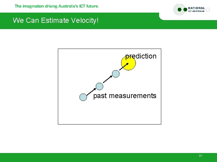
We Can Estimate Velocity! prediction past measurements 21

Points moving with constant velocity • We have – (the Greek letters denote noise terms) • Stack (u, v) into a single state vector – which is the form we had above 22

Points moving with constant acceleration • We have – (the Greek letters denote noise terms) • Stack (u, v, a) into a single state vector – which is the form we had above 23

24

25

Outline • • Motivation Tracking in Linear Dynamic Models The Kalman Filter (KF) KF for Nonlinear models 26

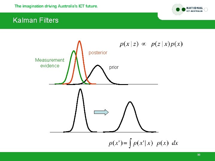
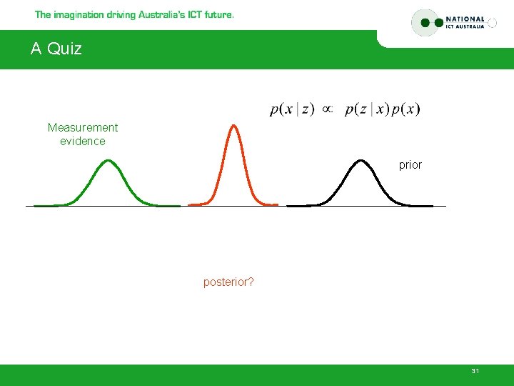
The Kalman Filter • Key ideas: – Linear models interact uniquely well with Gaussian noise - make the prior Gaussian, everything else Gaussian and the calculations are easy – Gaussians are really easy to represent --- once you know the mean and covariance, you’re done 27

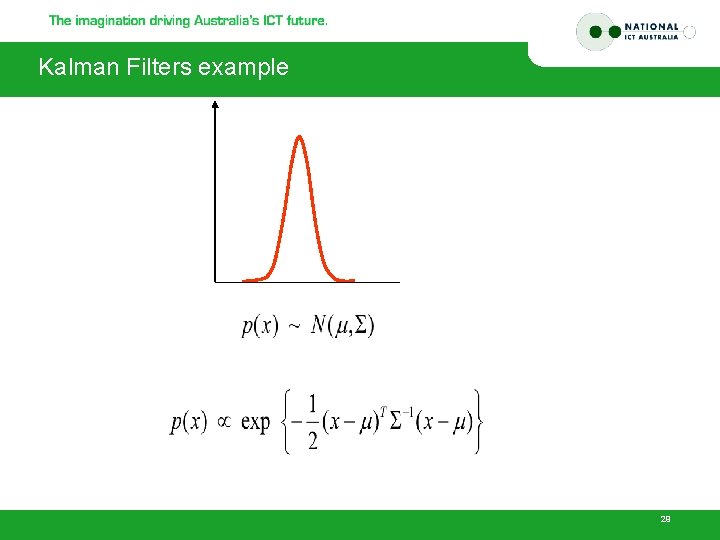
Kalman Filters example 29

Kalman Filters posterior Measurement evidence prior 30

A Quiz Measurement evidence prior posterior? 31

Kalman, Better! initial position prediction measurement update next prediciton 32

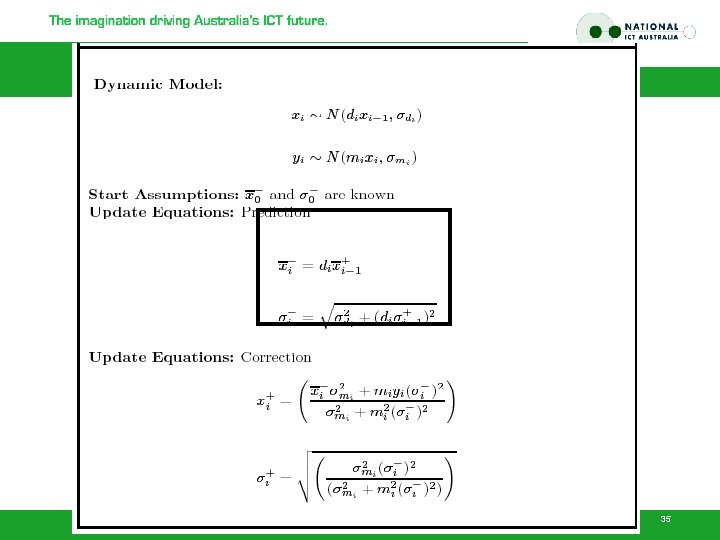
The Kalman Filter in 1 D • Dynamic Model • Notation Predicted mean Corrected mean 33

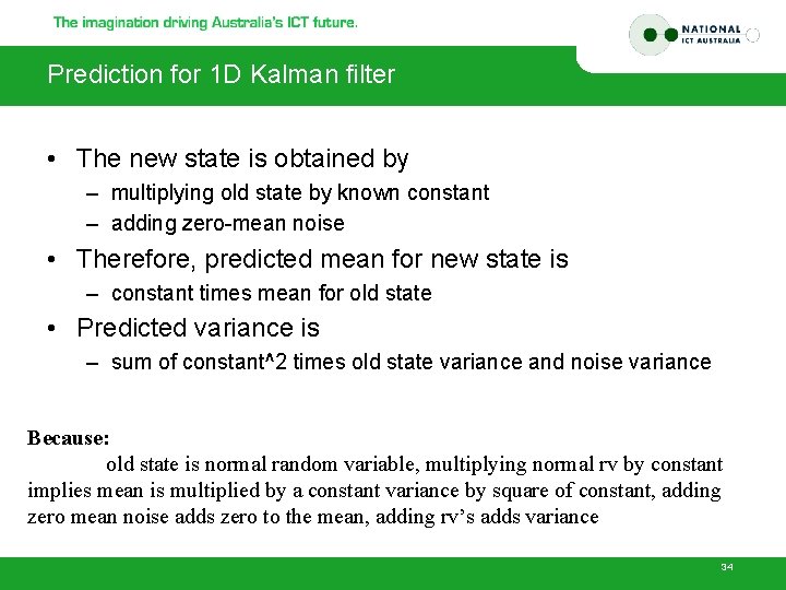
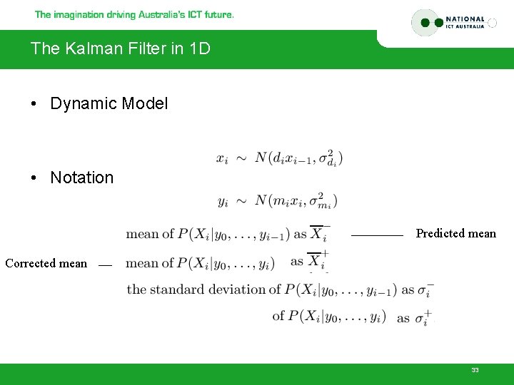
Prediction for 1 D Kalman filter • The new state is obtained by – multiplying old state by known constant – adding zero-mean noise • Therefore, predicted mean for new state is – constant times mean for old state • Predicted variance is – sum of constant^2 times old state variance and noise variance Because: old state is normal random variable, multiplying normal rv by constant implies mean is multiplied by a constant variance by square of constant, adding zero mean noise adds zero to the mean, adding rv’s adds variance 34

35

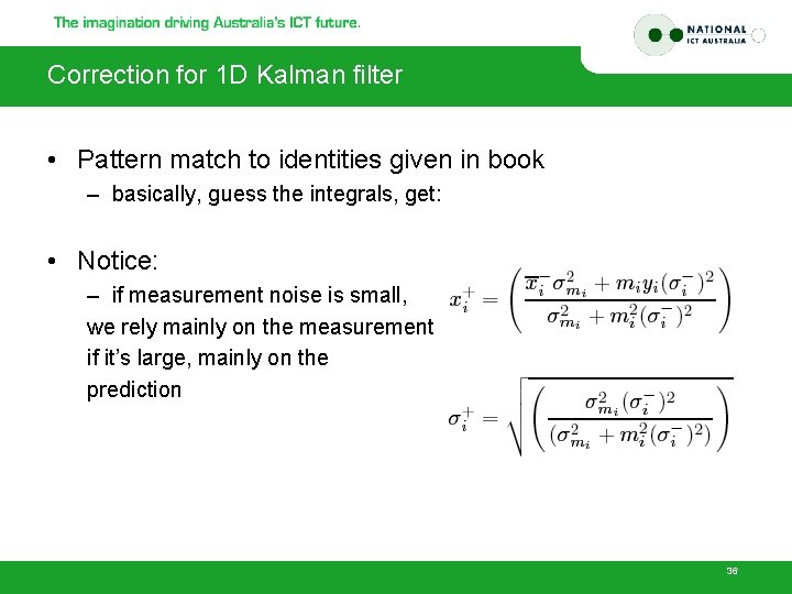
Correction for 1 D Kalman filter • Pattern match to identities given in book – basically, guess the integrals, get: • Notice: – if measurement noise is small, we rely mainly on the measurement, if it’s large, mainly on the prediction 36

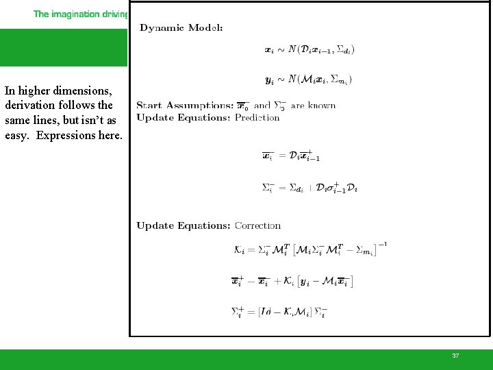
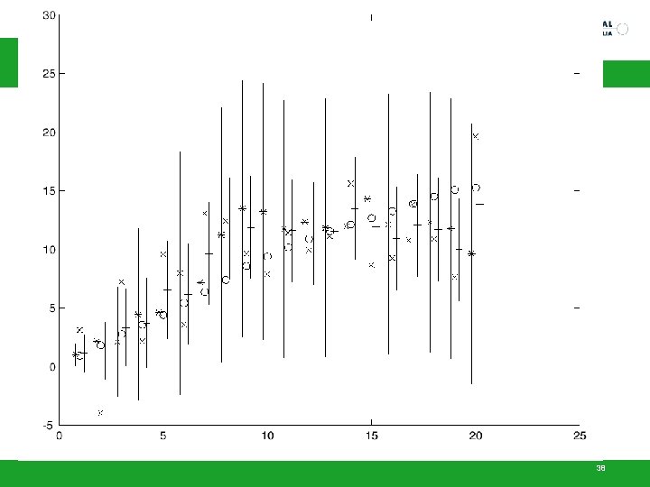
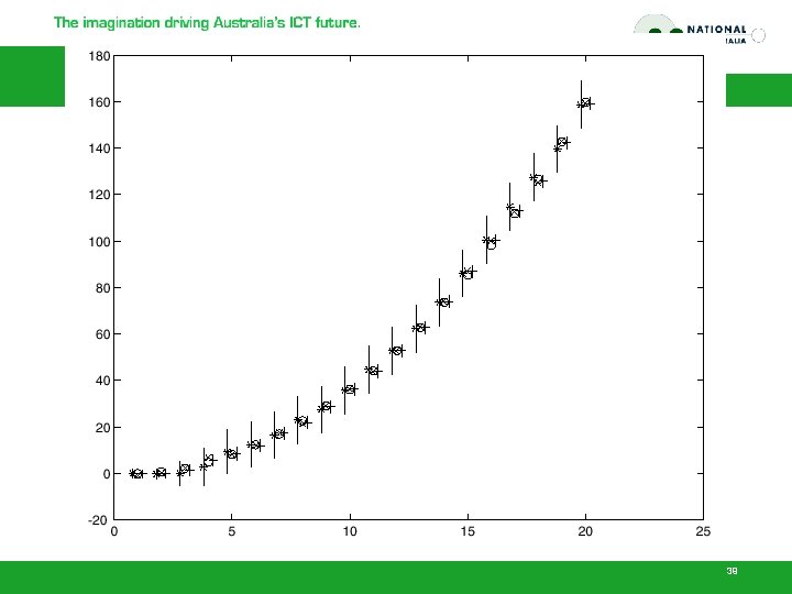
In higher dimensions, derivation follows the same lines, but isn’t as easy. Expressions here. 37

38

39

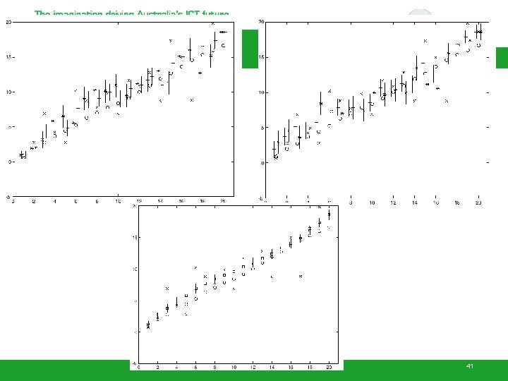
Smoothing • Idea – We don’t have the best estimate of state - what about the future? – Run two filters, one moving forward, the other backward in time. – Now combine state estimates • The crucial point here is that we can obtain a smoothed estimate by viewing the backward filter’s prediction as yet another measurement for the forward filter – so we’ve already done the equations 40

41

Data Association • Nearest neighbours – choose the measurement with highest probability given predicted state – popular, but can lead to catastrophe • Probabilistic Data Association – combine measurements, weighting by probability given predicted state – gate using predicted state 42

Outline • • Motivation Tracking in Linear Dynamic Models The Kalman Filter (KF) KF for Nonlinear models 43

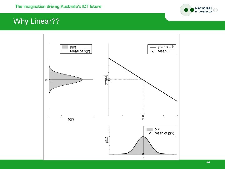
Why Linear? ? 44

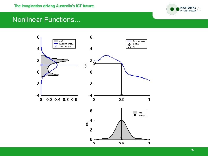
Nonlinear Functions… 45

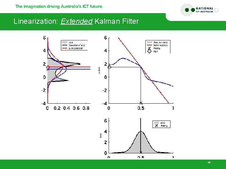
Linearization: Extended Kalman Filter 46

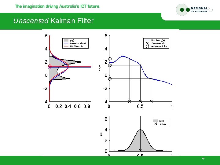
Unscented Kalman Filter 47

• Acknowledgement – Portion of slides drawn from the slides by David A. Forsyth – Portion of slides drawn from the Lec 12/CS 223 at Stanford Uni. – Video clips from PTI • Main References – “Computer Vision – A Modern Approach”, D. Forsyth & , 2002 – “An Introduction to Kalman filter”, G. Welch & G. Bishop, 2001 – “Robust car tracking using Kalman filtering and Bayesian templates” , F. Dellaert & C. Thorpe, 1997 – “Filter/Motion Tracking” (taught as Lecture 12 of CS 223 at Stanford), S. Thrun, R. Szeliski , H. Dhlkamp & D. Morris, 2005 48