Trace alignment with dynamic programming Chris Liner and

Trace alignment with dynamic programming Chris Liner and Bob Clapp SEP 115 Pg. 337 -345

Outline • Dynamic programming • Needleman-Wunsch • Seismic extensions

Dynamic programming • Solve non-linear problem • Works for non-linear problems that can be characterized as a series of decisions with a limited (discrete) set of outcomes • The best solution is built by finding the path that gives the maximum “score”

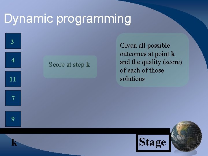
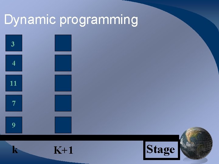
Dynamic programming 3 4 11 Score at step k Given all possible outcomes at point k and the quality (score) of each of those solutions 7 9 k Stage

Dynamic programming 3 4 11 7 9 k K+1 Stage

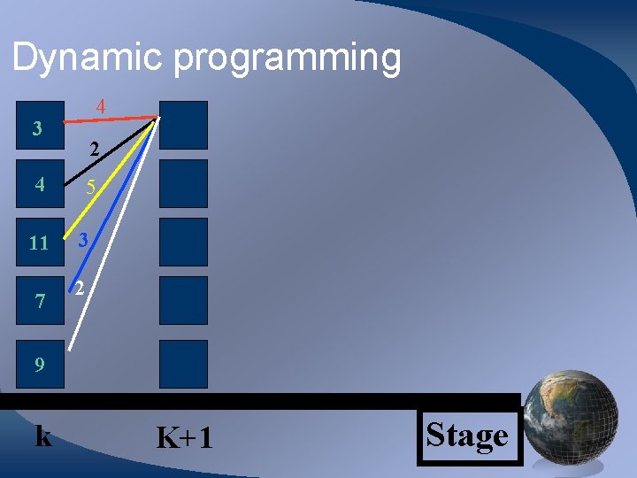
Dynamic programming 4 3 2 4 11 7 5 3 2 9 k K+1 Stage

Dynamic programming 4 3 2 4 + 5 11 7 3 2 9 k K+1 Stage

Dynamic programming 4 3 16 2 4 + 5 11 7 3 2 9 k K+1 Stage

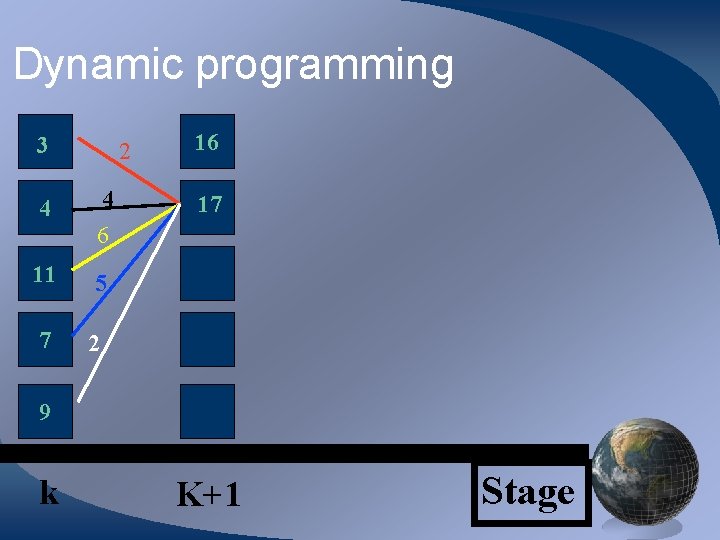
Dynamic programming 3 2 4 4 6 11 5 7 2 16 17 9 k K+1 Stage

Dynamic programming 3 2 4 4 +6 11 5 7 2 16 17 9 k K+1 Stage

Dynamic programming 3 16 4 17 11 13 7 10 9 10 k K+1 Stage

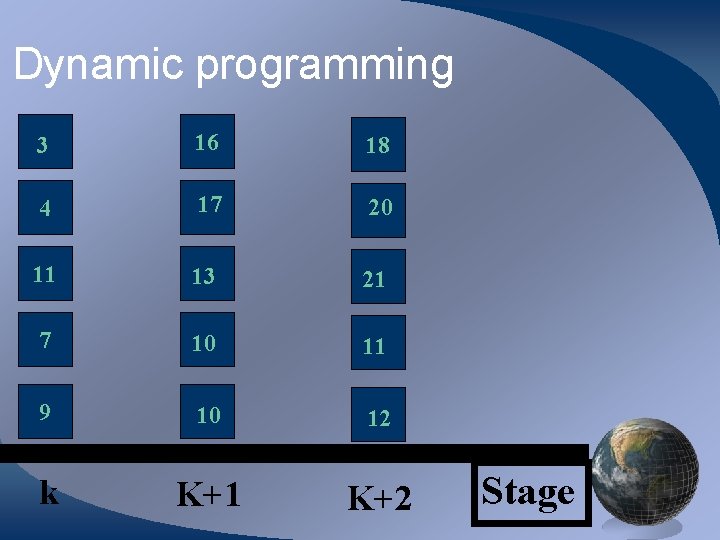
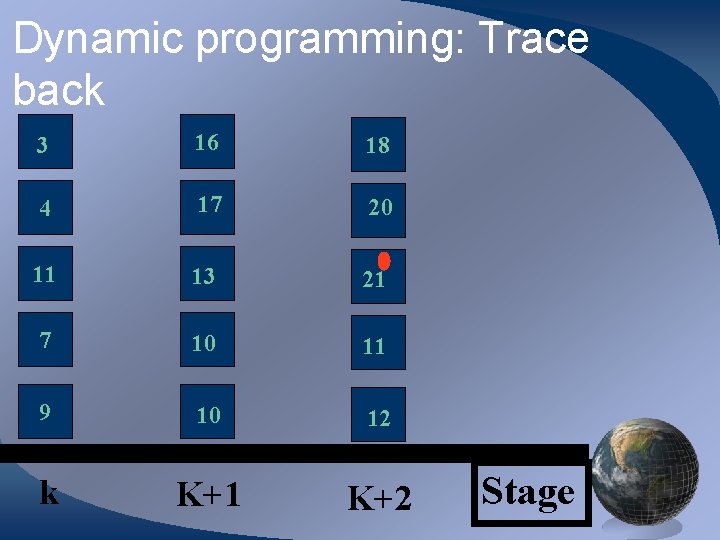
Dynamic programming 3 16 18 4 17 20 11 13 21 7 10 11 9 10 12 k K+1 K+2 Stage

Dynamic programming: Trace back 3 16 18 4 17 20 11 13 21 7 10 11 9 10 12 k K+1 K+2 Stage

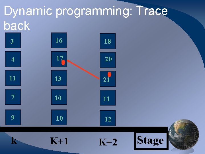
Dynamic programming: Trace back 3 16 18 4 17 20 11 13 21 7 10 11 9 10 12 k K+1 K+2 Stage

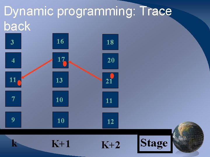
Dynamic programming: Trace back 3 16 18 4 17 20 11 13 21 7 10 11 9 10 12 k K+1 K+2 Stage

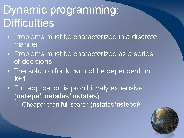
Dynamic programming: Difficulties • Problems must be characterized in a discrete manner • Problems must be characterized as a series of decisions • The solution for k can not be dependent on k+1 • Full application is prohibitively expensive (nsteps* nstates*nstates) – Cheaper than full search (nstates*nsteps)2

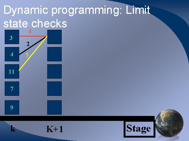
Dynamic programming: Limit state checks 3 4 4 2 5 11 7 9 k K+1 Stage

Outline • Dynamic programming • Needleman-Wunsch • Seismic extensions

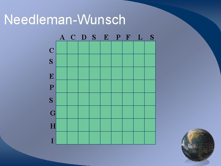
Needleman-Wunsch A C D S E C S E P S G H I P F L S

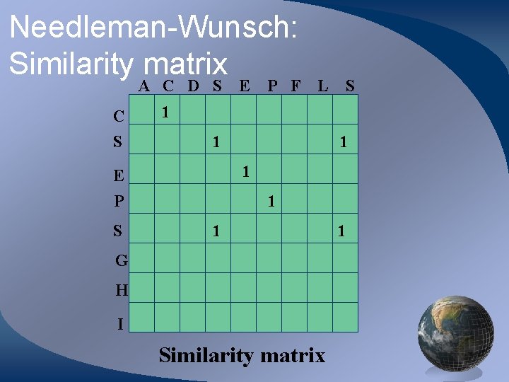
Needleman-Wunsch: Similarity matrix A C D S E C S L S 1 1 E P S P F 1 1 G H I Similarity matrix 1

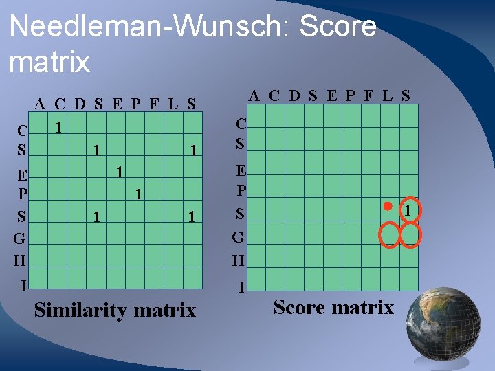
Needleman-Wunsch: Score matrix A C D S E P F L S 1 C S 1 1 1 E P 1 S 1 1 G H I A C D S E P F L S C S E P S G H I Similarity matrix Score matrix

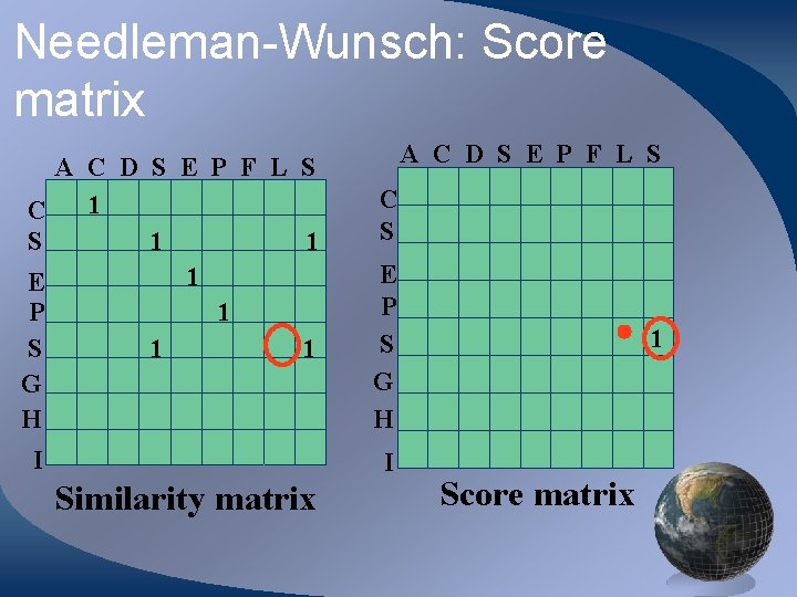
Needleman-Wunsch: Score matrix A C D S E P F L S 1 C S 1 1 1 E P 1 S 1 1 G H I A C D S E P F L S C S E P S G H I Similarity matrix 1 Score matrix

Needleman-Wunsch: Score matrix A C D S E P F L S 1 C S 1 1 1 E P 1 S 1 1 G H I A C D S E P F L S C S E P S G H I Similarity matrix 1 Score matrix

Needleman-Wunsch: Score matrix A C D S E P F L S 1 C S 1 1 1 E P 1 S 1 1 G H I A C D S E P F L S C S E P S G H I Similarity matrix 1 Score matrix

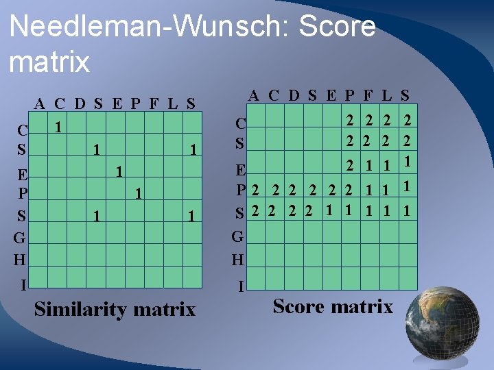
Needleman-Wunsch: Score matrix A C D S E P F L S 1 C S 1 1 1 E P 1 S 1 1 G H I A C D S E P F L S 2 2 2 E P 2 2 2 S 2 2 1 1 G H C S I Similarity matrix 2 2 1 1 1 Score matrix 2 2 1 1 1

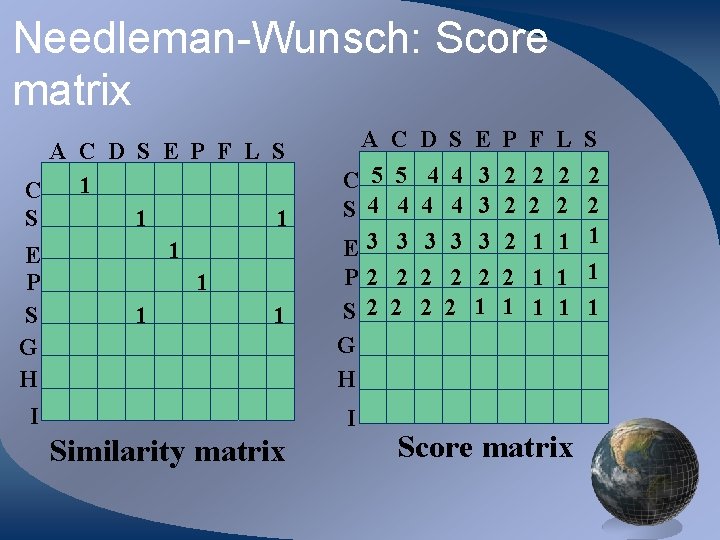
Needleman-Wunsch: Score matrix A C D S E P F L S 1 C S 1 1 1 E P 1 S 1 1 G H I A C D S E P F L S C 5 S 4 E 3 P 2 S 2 G H I Similarity matrix 5 4 3 2 2 4 4 3 3 2 2 3 3 3 2 1 2 2 1 1 1 Score matrix 2 2 1 1 1

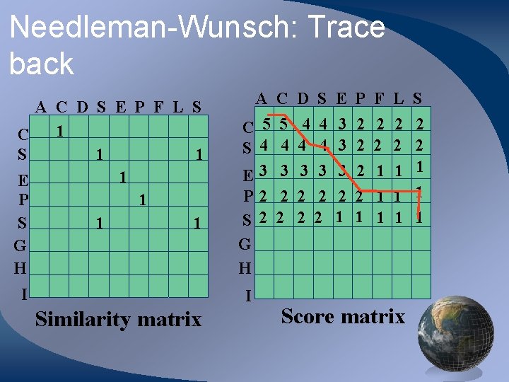
Needleman-Wunsch: Trace back A C D S E P F L S 1 C S 1 1 1 E P 1 S 1 1 G H I A C D S E P F L S C 5 S 4 E 3 P 2 S 2 G H I Similarity matrix 5 4 3 2 2 4 4 3 3 2 2 3 3 3 2 1 2 2 1 1 1 Score matrix 2 2 1 1 1

Needleman-Wunsch • Our states are the various matches • Our decision is whether to move diagonal, horizontally, or vertically through the matrix • We are cutting costs by checking only those three states at each decision

Outline • Dynamic programming • Needleman-Wunsch • Seismic extensions

Windowed correlation for similarity matrix x(i) - trace 1 y(j) - trace 2 S(i, j) - similarity matrix n - correlation length

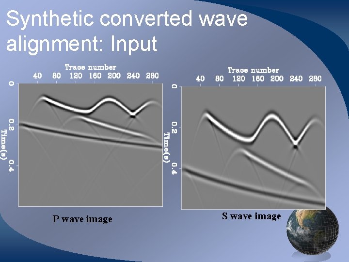
Synthetic converted wave alignment: Input P wave image S wave image

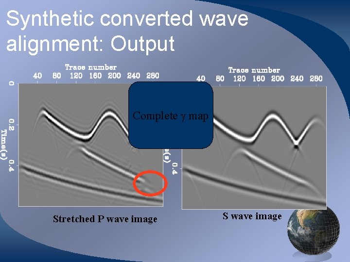
Synthetic converted wave alignment: Output Complete map Stretched P wave image S wave image

Gather alignment d - non-aligned gather m - aligned gather - smoothness parameter L - Mapping operator from alignment A - Non-stationary PEF estimated from data operator

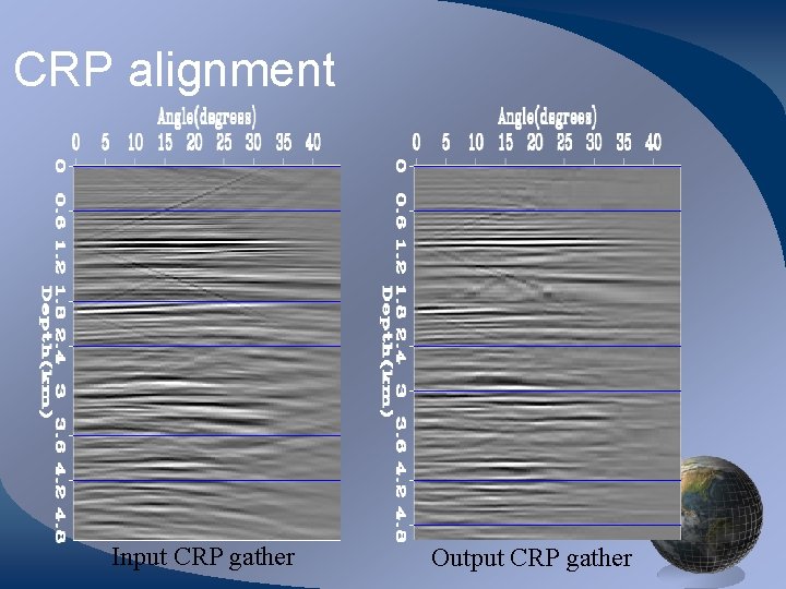
CRP alignment Input CRP gather Output CRP gather

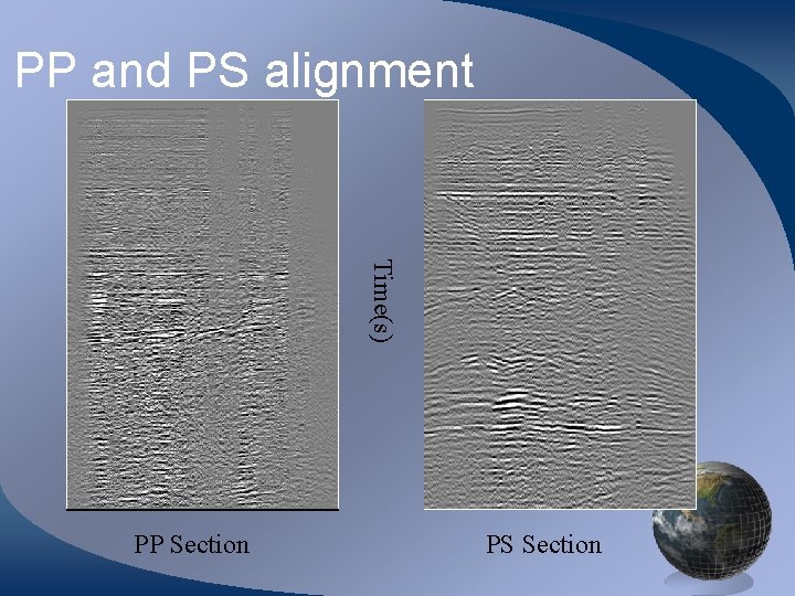
PP and PS alignment Time(s) PP Section PS Section

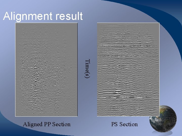
Alignment result Time(s) Aligned PP Section PS Section

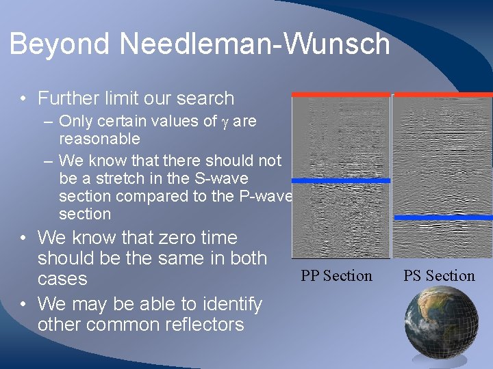
Beyond Needleman-Wunsch • Further limit our search – Only certain values of are reasonable – We know that there should not be a stretch in the S-wave section compared to the P-wave section • We know that zero time should be the same in both cases • We may be able to identify other common reflectors PP Section PS Section

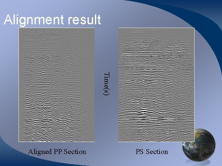
Alignment result Time(s) Aligned PP Section PS Section

Alignment result Time(s) Aligned PP Section Poor PP alignment

Conclusions • Dynamic programming can be an effective tool for solving certain classes of problems • For simple alignment problems Needlman-Wunsch is an effective alignment tool • For more complex problems additional constraints need to be added