TP 15 Tracking Computer Vision FCUP 2013 Miguel

TP 15 - Tracking Computer Vision, FCUP, 2013 Miguel Coimbra Slides by Prof. Kristen Grauman

Outline • Today: Tracking – – Tracking as inference Linear models of dynamics Kalman filters General challenges in tracking

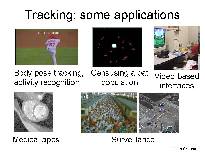
Tracking: some applications Body pose tracking, Censusing a bat Video-based activity recognition population interfaces Medical apps Surveillance Kristen Grauman

Why is tracking challenging?

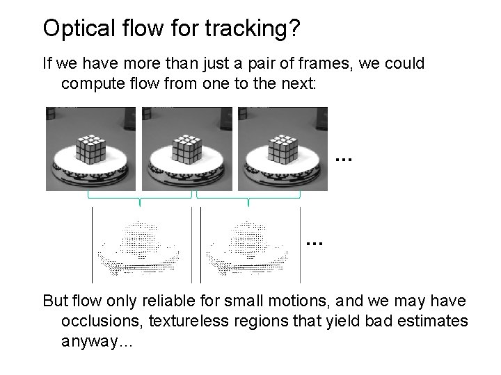
Optical flow for tracking? If we have more than just a pair of frames, we could compute flow from one to the next: … … But flow only reliable for small motions, and we may have occlusions, textureless regions that yield bad estimates anyway…

Motion estimation techniques • Direct methods • Directly recover image motion at each pixel from spatio-temporal image brightness variations • Dense motion fields, but sensitive to appearance variations • Suitable for video and when image motion is small • Feature-based methods • Extract visual features (corners, textured areas) and track them over multiple frames • Sparse motion fields, but more robust tracking • Suitable when image motion is large (10 s of pixels)

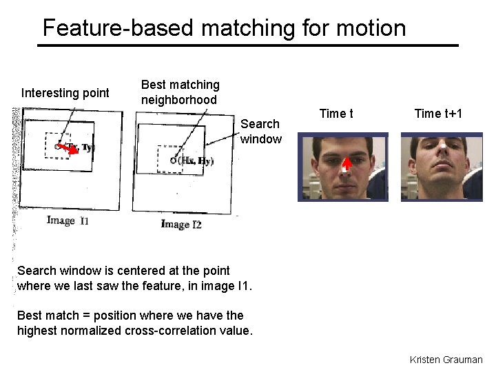
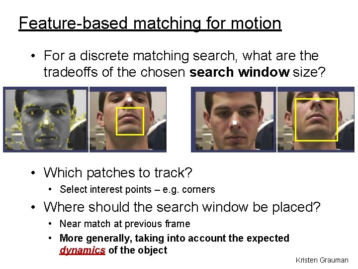
Feature-based matching for motion Interesting point Best matching neighborhood Search window Time t+1 Search window is centered at the point where we last saw the feature, in image I 1. Best match = position where we have the highest normalized cross-correlation value. Kristen Grauman

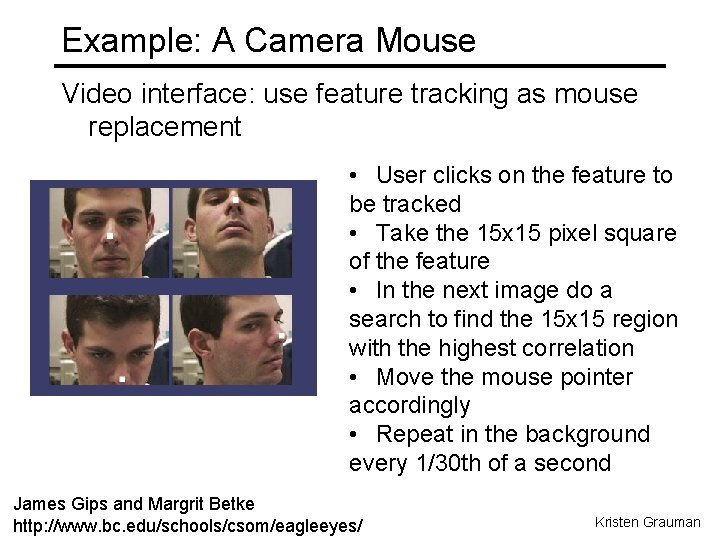
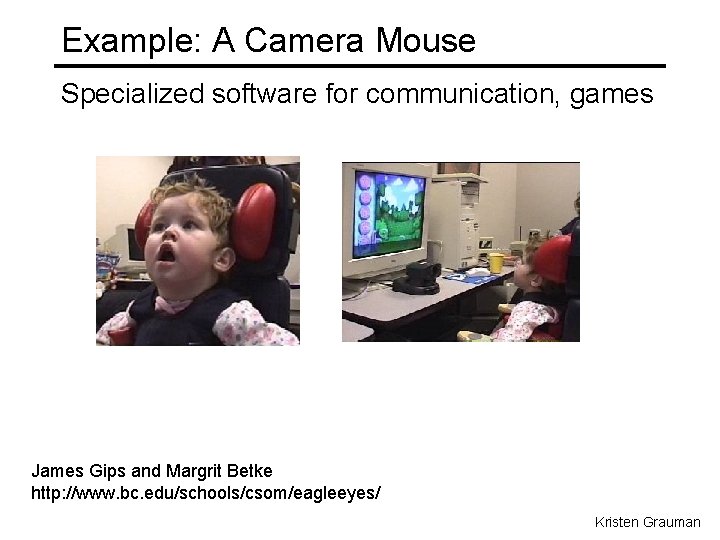
Example: A Camera Mouse Video interface: use feature tracking as mouse replacement • User clicks on the feature to be tracked • Take the 15 x 15 pixel square of the feature • In the next image do a search to find the 15 x 15 region with the highest correlation • Move the mouse pointer accordingly • Repeat in the background every 1/30 th of a second James Gips and Margrit Betke http: //www. bc. edu/schools/csom/eagleeyes/ Kristen Grauman

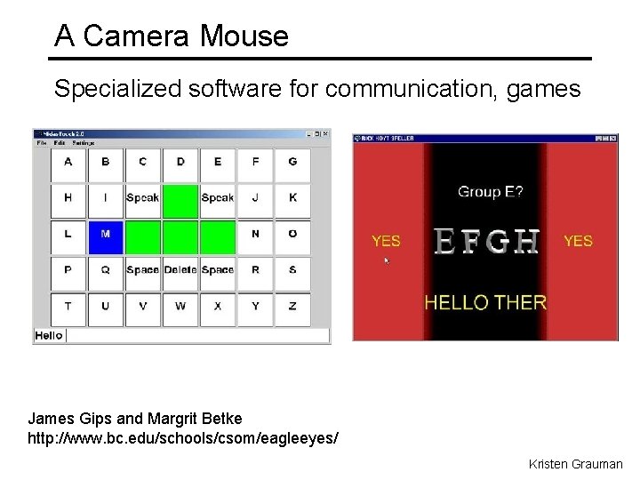
Example: A Camera Mouse Specialized software for communication, games James Gips and Margrit Betke http: //www. bc. edu/schools/csom/eagleeyes/ Kristen Grauman

A Camera Mouse Specialized software for communication, games James Gips and Margrit Betke http: //www. bc. edu/schools/csom/eagleeyes/ Kristen Grauman

Feature-based matching for motion • For a discrete matching search, what are the tradeoffs of the chosen search window size? • Which patches to track? • Select interest points – e. g. corners • Where should the search window be placed? • Near match at previous frame • More generally, taking into account the expected dynamics of the object Kristen Grauman

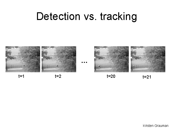
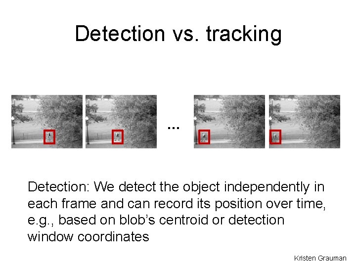
Detection vs. tracking … t=1 t=20 t=21 Kristen Grauman

Detection vs. tracking … Detection: We detect the object independently in each frame and can record its position over time, e. g. , based on blob’s centroid or detection window coordinates Kristen Grauman

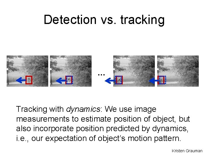
Detection vs. tracking … Tracking with dynamics: We use image measurements to estimate position of object, but also incorporate position predicted by dynamics, i. e. , our expectation of object’s motion pattern. Kristen Grauman

Detection vs. tracking … Tracking with dynamics: We use image measurements to estimate position of object, but also incorporate position predicted by dynamics, i. e. , our expectation of object’s motion pattern. Kristen Grauman

Tracking with dynamics • Use model of expected motion to predict where objects will occur in next frame, even before seeing the image. • Intent: – Do less work looking for the object, restrict the search. – Get improved estimates since measurement noise is tempered by smoothness, dynamics priors. • Assumption: continuous motion patterns: – Camera is not moving instantly to new viewpoint – Objects do not disappear and reappear in different places in the scene – Gradual change in pose between camera and scene Kristen Grauman

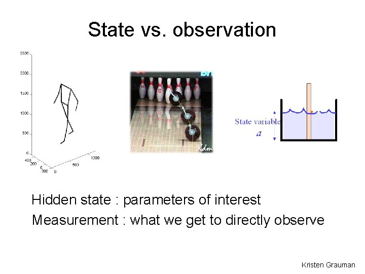
Tracking as inference • The hidden state consists of the true parameters we care about, denoted X. • The measurement is our noisy observation that results from the underlying state, denoted Y. • At each time step, state changes (from Xt-1 to Xt ) and we get a new observation Yt. Kristen Grauman

State vs. observation Hidden state : parameters of interest Measurement : what we get to directly observe Kristen Grauman

Tracking as inference • The hidden state consists of the true parameters we care about, denoted X. • The measurement is our noisy observation that results from the underlying state, denoted Y. • At each time step, state changes (from Xt-1 to Xt ) and we get a new observation Yt. • Our goal: recover most likely state Xt given – All observations seen so far. – Knowledge about dynamics of state transitions. Kristen Grauman

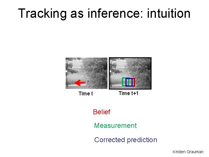
Tracking as inference: intuition Time t+1 Time t Belief Measurement Corrected prediction Kristen Grauman

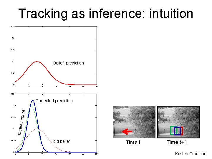
Tracking as inference: intuition measurement Belief: prediction measu rement Corrected prediction old belief Time t+1 Kristen Grauman

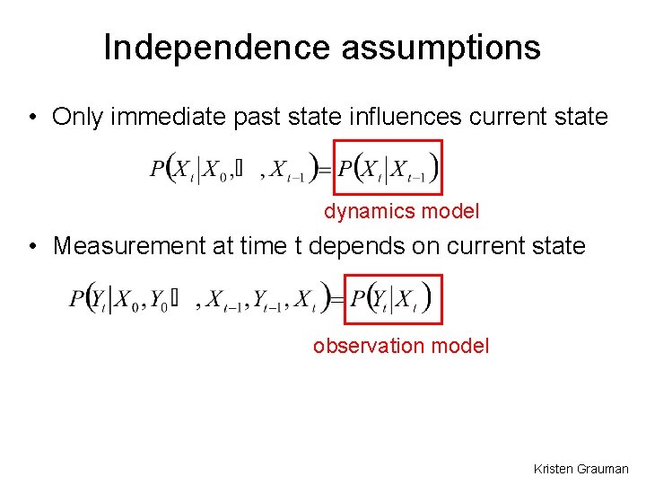
Independence assumptions • Only immediate past state influences current state dynamics model • Measurement at time t depends on current state observation model Kristen Grauman

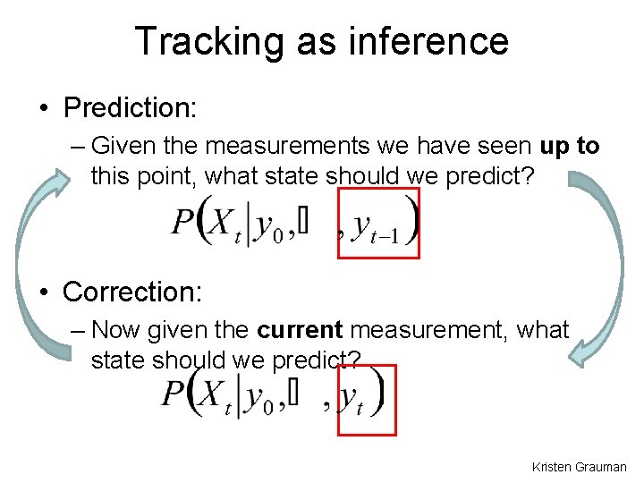
Tracking as inference • Prediction: – Given the measurements we have seen up to this point, what state should we predict? • Correction: – Now given the current measurement, what state should we predict? Kristen Grauman

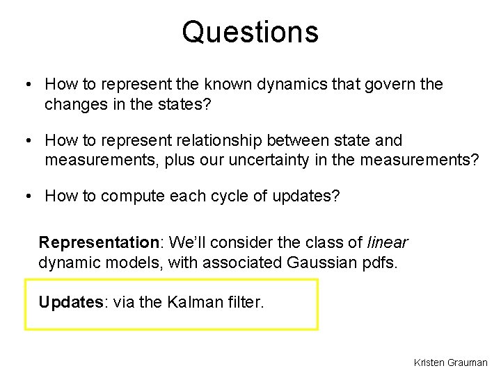
Questions • How to represent the known dynamics that govern the changes in the states? • How to represent relationship between state and measurements, plus our uncertainty in the measurements? • How to compute each cycle of updates? Representation: We’ll consider the class of linear dynamic models, with associated Gaussian pdfs. Updates: via the Kalman filter. Kristen Grauman

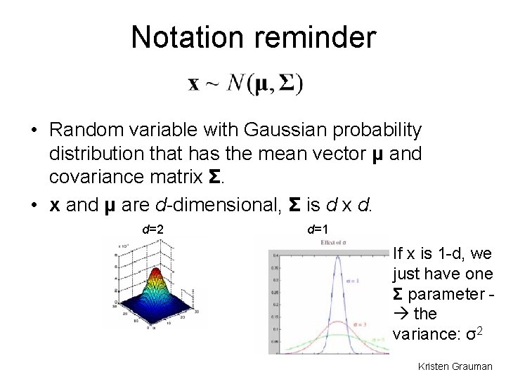
Notation reminder • Random variable with Gaussian probability distribution that has the mean vector μ and covariance matrix Σ. • x and μ are d-dimensional, Σ is d x d. d=2 d=1 If x is 1 -d, we just have one Σ parameter the variance: σ2 Kristen Grauman

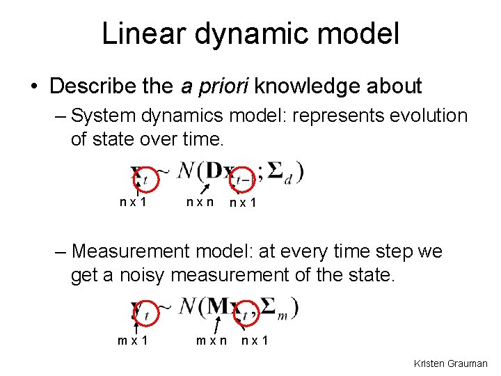
Linear dynamic model • Describe the a priori knowledge about – System dynamics model: represents evolution of state over time. nx 1 nxn nx 1 – Measurement model: at every time step we get a noisy measurement of the state. mx 1 mxn nx 1 Kristen Grauman

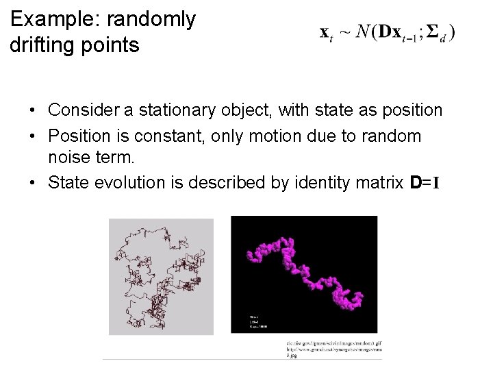
Example: randomly drifting points • Consider a stationary object, with state as position • Position is constant, only motion due to random noise term. • State evolution is described by identity matrix D=I

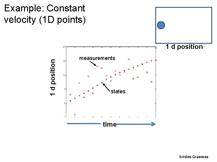
Example: Constant velocity (1 D points) 1 d position measurements states time Kristen Grauman

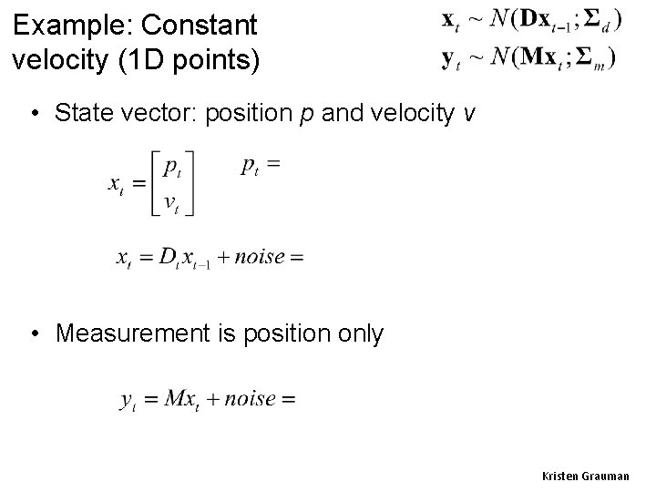
Example: Constant velocity (1 D points) • State vector: position p and velocity v • Measurement is position only Kristen Grauman

Questions • How to represent the known dynamics that govern the changes in the states? • How to represent relationship between state and measurements, plus our uncertainty in the measurements? • How to compute each cycle of updates? Representation: We’ll consider the class of linear dynamic models, with associated Gaussian pdfs. Updates: via the Kalman filter. Kristen Grauman

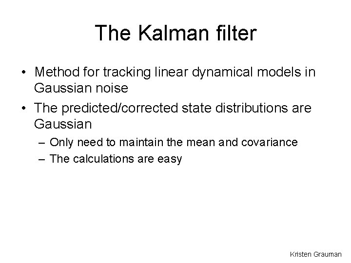
The Kalman filter • Method for tracking linear dynamical models in Gaussian noise • The predicted/corrected state distributions are Gaussian – Only need to maintain the mean and covariance – The calculations are easy Kristen Grauman

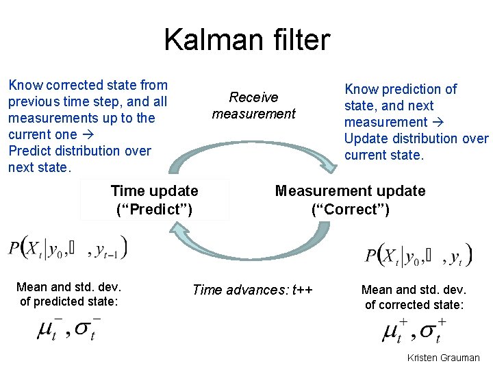
Kalman filter Know corrected state from previous time step, and all measurements up to the current one Predict distribution over next state. Receive measurement Time update (“Predict”) Mean and std. dev. of predicted state: Know prediction of state, and next measurement Update distribution over current state. Measurement update (“Correct”) Time advances: t++ Mean and std. dev. of corrected state: Kristen Grauman

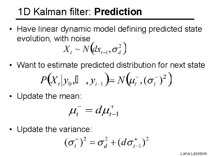
1 D Kalman filter: Prediction • Have linear dynamic model defining predicted state evolution, with noise • Want to estimate predicted distribution for next state • Update the mean: • Update the variance: Lana Lazebnik

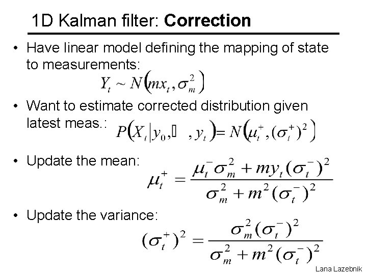
1 D Kalman filter: Correction • Have linear model defining the mapping of state to measurements: • Want to estimate corrected distribution given latest meas. : • Update the mean: • Update the variance: Lana Lazebnik

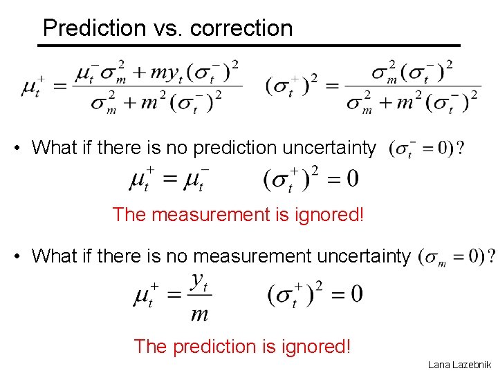
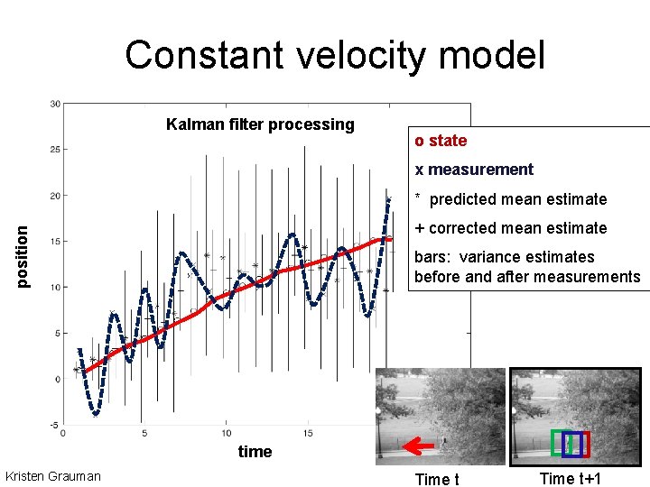
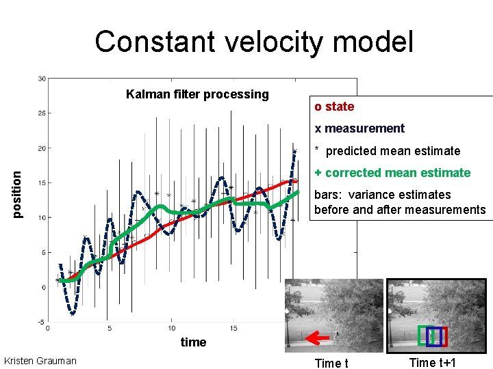
Prediction vs. correction • What if there is no prediction uncertainty The measurement is ignored! • What if there is no measurement uncertainty The prediction is ignored! Lana Lazebnik

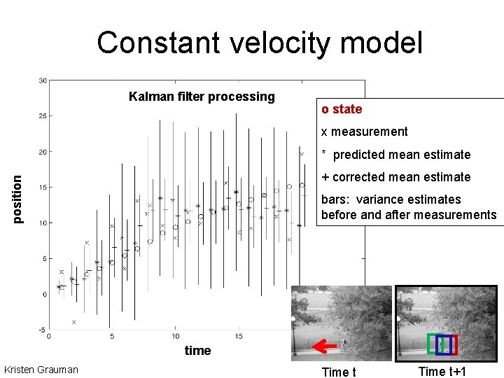
Constant velocity model Kalman filter processing o state x measurement * predicted mean estimate position + corrected mean estimate bars: variance estimates before and after measurements time Kristen Grauman Time t+1

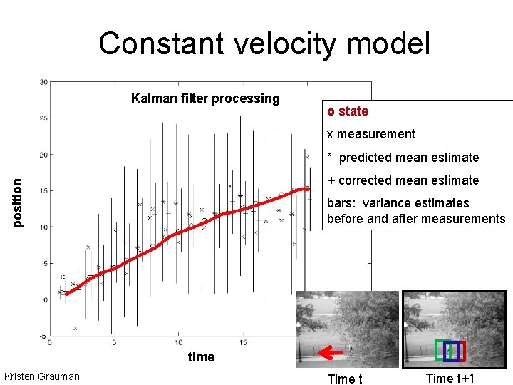
Constant velocity model Kalman filter processing o state x measurement * predicted mean estimate position + corrected mean estimate bars: variance estimates before and after measurements time Kristen Grauman Time t+1

Constant velocity model Kalman filter processing o state x measurement * predicted mean estimate position + corrected mean estimate bars: variance estimates before and after measurements time Kristen Grauman Time t+1

Constant velocity model Kalman filter processing o state x measurement * predicted mean estimate position + corrected mean estimate bars: variance estimates before and after measurements time Kristen Grauman Time t+1

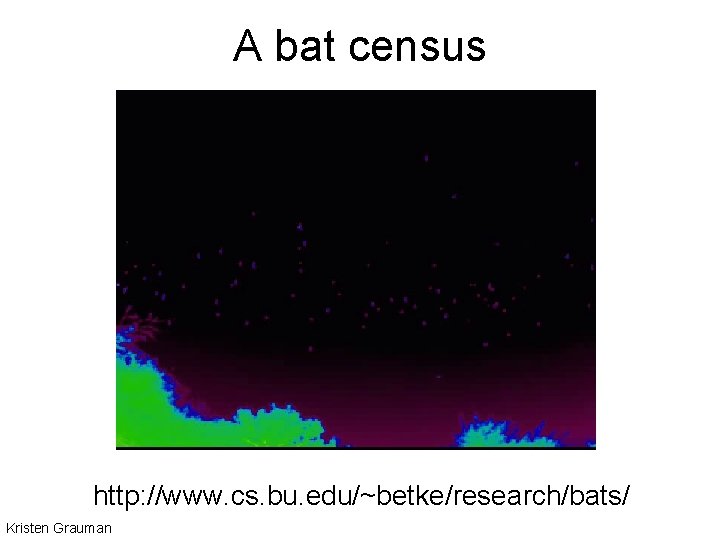
• http: //www. cs. bu. edu/~betke/research/bats/ Kristen Grauman

A bat census http: //www. cs. bu. edu/~betke/research/bats/ Kristen Grauman

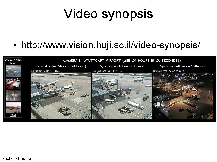
Video synopsis • http: //www. vision. huji. ac. il/video-synopsis/ Kristen Grauman

Tracking: issues • Initialization – Often done manually – Background subtraction, detection can also be used • Data association, multiple tracked objects – Occlusions, clutter

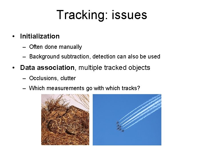
Tracking: issues • Initialization – Often done manually – Background subtraction, detection can also be used • Data association, multiple tracked objects – Occlusions, clutter – Which measurements go with which tracks?

Tracking: issues • Initialization – Often done manually – Background subtraction, detection can also be used • Data association, multiple tracked objects – Occlusions, clutter • Deformable and articulated objects

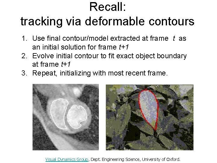
Recall: tracking via deformable contours 1. Use final contour/model extracted at frame t as an initial solution for frame t+1 2. Evolve initial contour to fit exact object boundary at frame t+1 3. Repeat, initializing with most recent frame. Visual Dynamics Group, Dept. Engineering Science, University of Oxford.

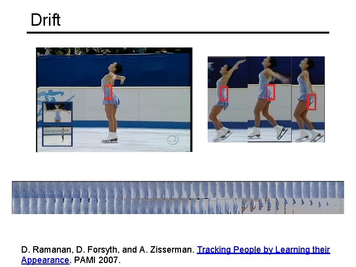
Tracking: issues • Initialization – Often done manually – Background subtraction, detection can also be used • Data association, multiple tracked objects – Occlusions, clutter • Deformable and articulated objects • Constructing accurate models of dynamics – E. g. , Fitting parameters for a linear dynamics model • Drift – Accumulation of errors over time

Drift D. Ramanan, D. Forsyth, and A. Zisserman. Tracking People by Learning their Appearance. PAMI 2007.

Summary • Tracking as inference – Goal: estimate posterior of object position given measurement • Linear models of dynamics – Represent state evolution and measurement models • Kalman filters – Recursive prediction/correction updates to refine measurement • General tracking challenges