Towards theoretical frameworks for comparing constraint satisfaction models

Towards theoretical frameworks for comparing constraint satisfaction models and algorithms Peter van Beek, University of Waterloo CP 2001 · Paphos, Cyprus November 2001

Acknowledgements Joint work with: Fahiem Bacchus Xinguang Chen Grzegorz Kondrak Toby Walsh 2 2

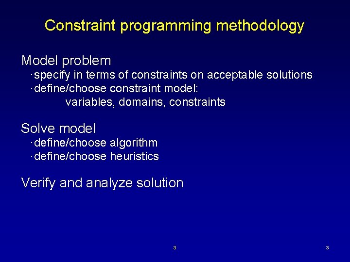
Constraint programming methodology Model problem ·specify in terms of constraints on acceptable solutions ·define/choose constraint model: variables, domains, constraints Solve model ·define/choose algorithm ·define/choose heuristics Verify and analyze solution 3 3

Previous work Many models, algorithms, and heuristics proposed Choice of model, algorithm, and heuristic can greatly influence efficiency (e. g. , Nadel, 1990; Ginsberg et al. , 1990; 1995 2001) Frost and Dechter, 1994; Tsang et al. , Smith et al. , 2000; Beacham et al. , 4 4

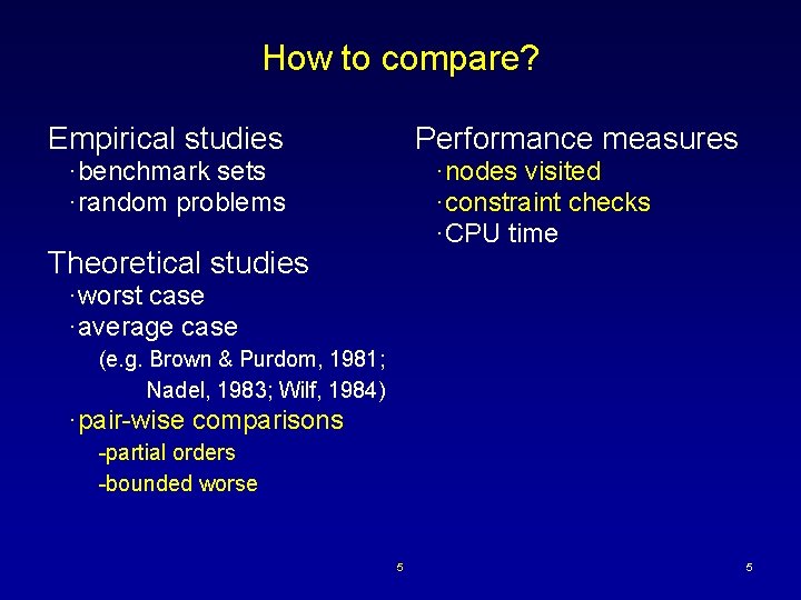
How to compare? Empirical studies Performance measures ·benchmark sets ·random problems ·nodes visited ·constraint checks ·CPU time Theoretical studies ·worst case ·average case (e. g. Brown & Purdom, 1981; Nadel, 1983; Wilf, 1984) ·pair-wise comparisons -partial orders -bounded worse 5 5

Part I Comparing backtracking algorithms 6 6

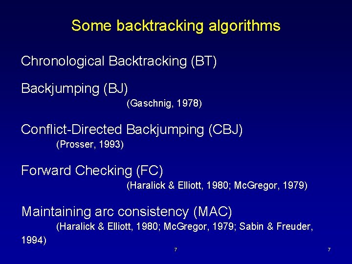
Some backtracking algorithms Chronological Backtracking (BT) Backjumping (BJ) (Gaschnig, 1978) Conflict-Directed Backjumping (CBJ) (Prosser, 1993) Forward Checking (FC) (Haralick & Elliott, 1980; Mc. Gregor, 1979) Maintaining arc consistency (MAC) (Haralick & Elliott, 1980; Mc. Gregor, 1979; Sabin & Freuder, 1994) 7 7

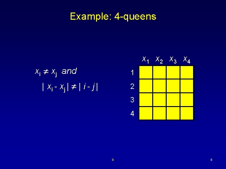
Example: 4 -queens x 1 x 2 x 3 x 4 xi xj and 1 | xi - xj | | i - j | 2 3 4 8 8

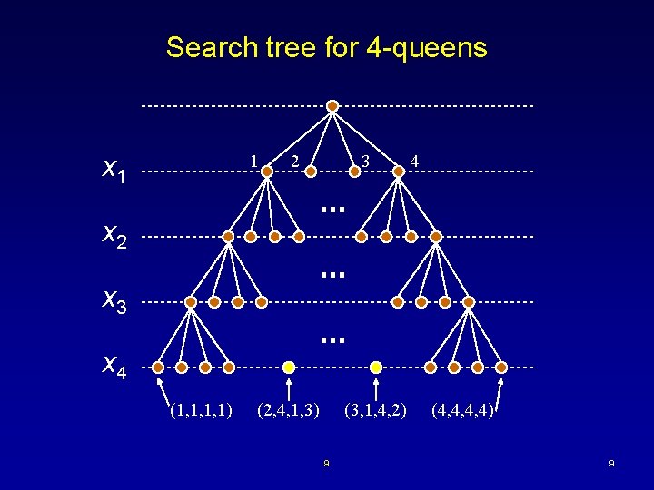
Search tree for 4 -queens x 1 1 2 3 4 x 2 x 3 x 4 (1, 1, 1, 1) (2, 4, 1, 3) (3, 1, 4, 2) 9 (4, 4, 4, 4) 9

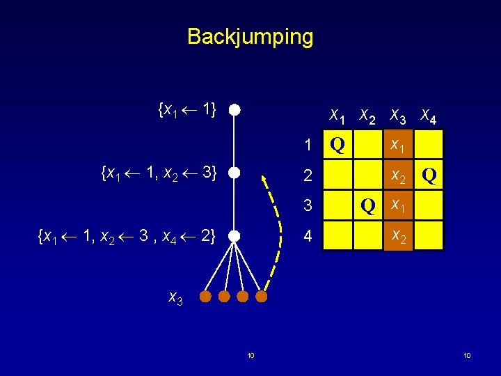
Backjumping {x 1 1} x 1 x 2 x 3 x 4 1 {x 1 1, x 2 3} 2 {x 1 1, x 2 3 , x 4 2} Q x 1 x 2 Q 3 Q x 1 4 x 2 x 3 10 10

“New” algorithms: BJ 1, …, BJn BJk : ·allowed to backjump at most k times from a leaf ·after that it must chronologically backtrack Special cases: ·BJ 1 equivalent to BJ ·BJn equivalent to CBJ 11 11

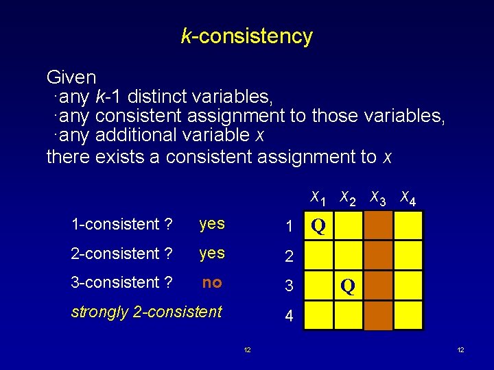
k-consistency Given ·any k-1 distinct variables, ·any consistent assignment to those variables, ·any additional variable x there exists a consistent assignment to x x 1 x 2 x 3 x 4 1 -consistent ? yes 1 2 -consistent ? yes 2 3 -consistent ? no 3 strongly 2 -consistent 4 12 Q Q 12

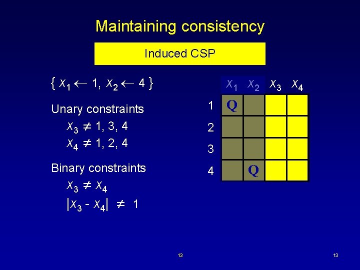
Maintaining consistency Induced CSP { x 1 1, x 2 4 } x 1 x 2 x 3 x 4 Unary constraints x 3 1, 3, 4 x 4 1, 2, 4 1 Binary constraints 4 Q 2 3 x 3 x 4 |x 3 - x 4| 1 13 Q 13

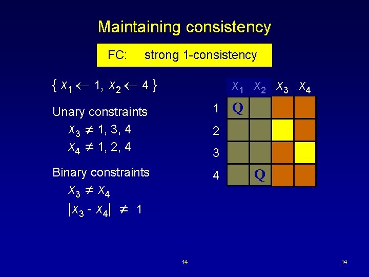
Maintaining consistency FC: strong 1 -consistency { x 1 1, x 2 4 } x 1 x 2 x 3 x 4 Unary constraints x 3 1, 3, 4 x 4 1, 2, 4 1 Binary constraints 4 Q 2 3 x 3 x 4 |x 3 - x 4| 1 14 Q 14

Maintaining consistency MAC: strong 2 -consistency { x 1 1, x 2 4 } x 1 x 2 x 3 x 4 Unary constraints x 3 1, 3, 4 x 4 1, 2, 4 1 Binary constraints 4 Q 2 3 x 3 x 4 |x 3 - x 4| 1 15 Q 15

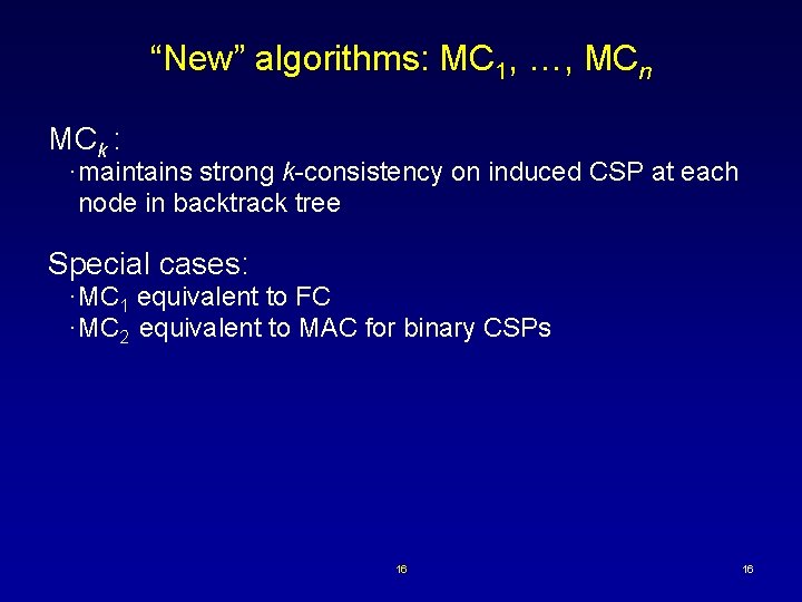
“New” algorithms: MC 1, …, MCn MCk : ·maintains strong k-consistency on induced CSP at each node in backtrack tree Special cases: ·MC 1 equivalent to FC ·MC 2 equivalent to MAC for binary CSPs 16 16

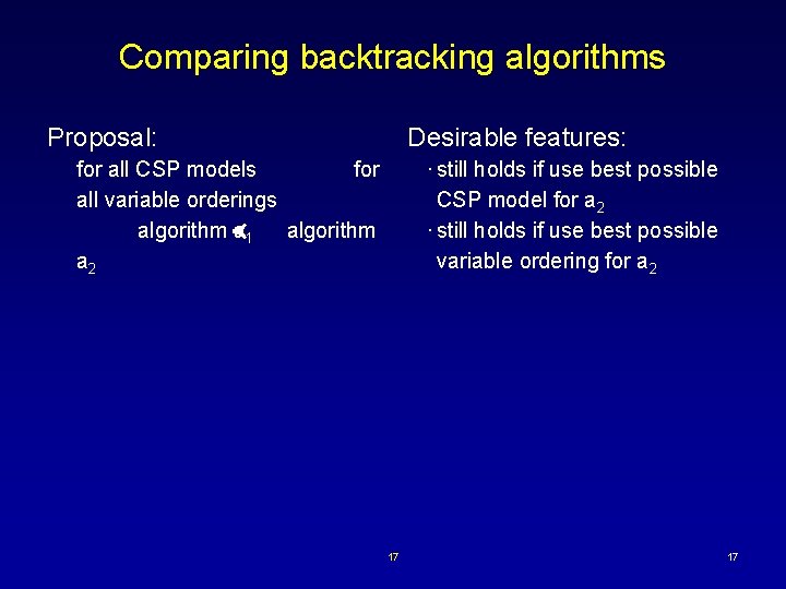
Comparing backtracking algorithms Proposal: Desirable features: · still holds if use best possible CSP model for a 2 · still holds if use best possible variable ordering for a 2 for all CSP models for all variable orderings algorithm a 1 algorithm a 2 17 17

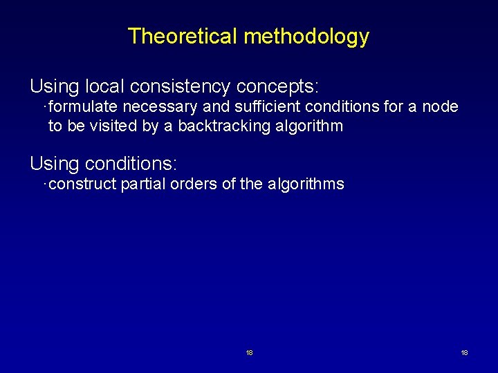
Theoretical methodology Using local consistency concepts: ·formulate necessary and sufficient conditions for a node to be visited by a backtracking algorithm Using conditions: ·construct partial orders of the algorithms 18 18

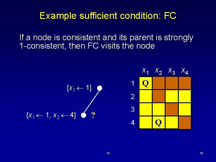
Example sufficient condition: FC If a node is consistent and its parent is strongly 1 -consistent, then FC visits the node x 1 x 2 x 3 x 4 1 {x 1 1} {x 1 1, x 2 4} Q 2 3 ? 4 19 Q 19

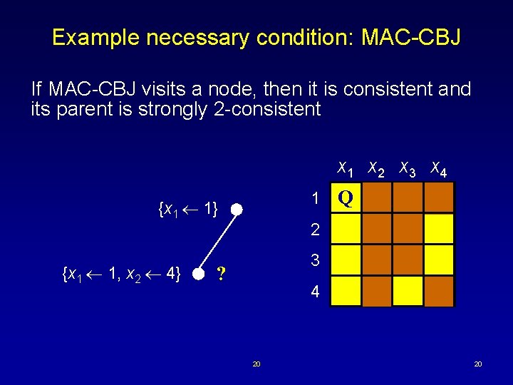
Example necessary condition: MAC-CBJ If MAC-CBJ visits a node, then it is consistent and its parent is strongly 2 -consistent x 1 x 2 x 3 x 4 1 {x 1 1} {x 1 1, x 2 4} Q 2 3 ? 4 20 20

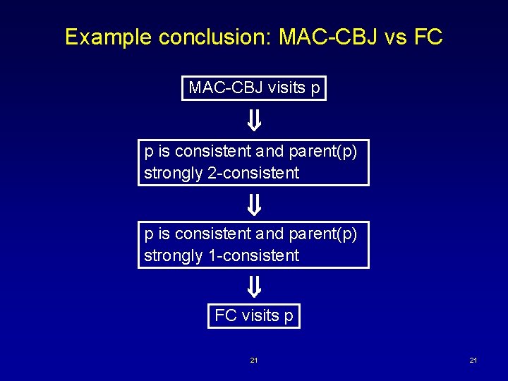
Example conclusion: MAC-CBJ vs FC MAC-CBJ visits p p is consistent and parent(p) strongly 2 -consistent p is consistent and parent(p) strongly 1 -consistent FC visits p 21 21

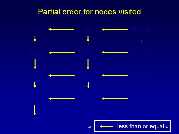
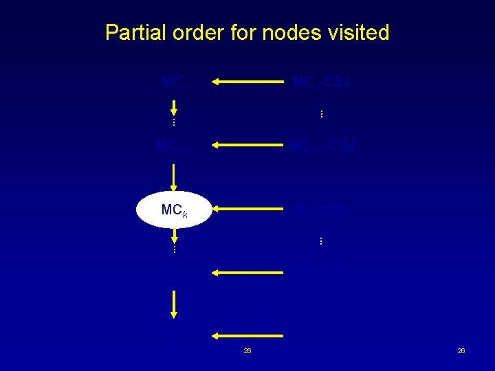
Partial order for nodes visited BJn MCn . . BJk+1 MCk+1 -CBJ BJk MCk-CBJ . . BJ 1 MC 1 BT 22 MCn-CBJ . . MC 1 -CBJ less than or equal 22

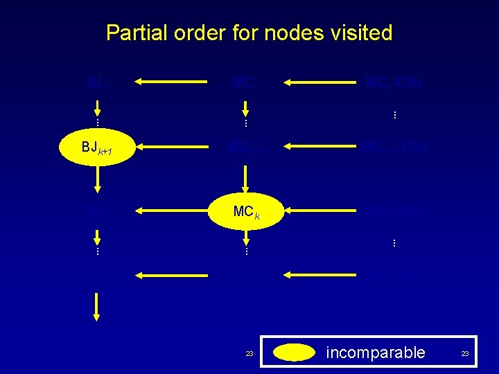
Partial order for nodes visited BJn MCn . . BJk+1 MCk+1 -CBJ BJk MCk-CBJ . . BJ 1 MC 1 BT 23 MCn-CBJ . . MC 1 -CBJ incomparable 23

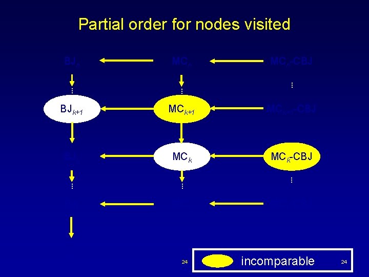
Partial order for nodes visited BJn MCn . . BJk+1 MCk+1 -CBJ BJk MCk-CBJ . . BJ 1 MC 1 BT 24 MCn-CBJ . . MC 1 -CBJ incomparable 24

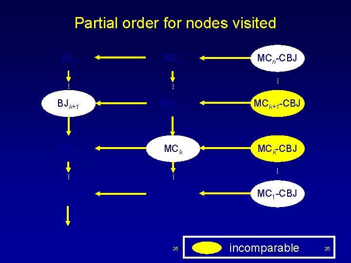
Partial order for nodes visited BJn MCn . . BJk+1 MCk+1 -CBJ BJk MCk-CBJ . . BJ 1 MC 1 BT 25 MCn-CBJ . . MC 1 -CBJ incomparable 25

Partial order for nodes visited MCn-CBJ . . MCk+1 -CBJ MCk-CBJ . . MC 1 -CBJ BT CBJ 26 26

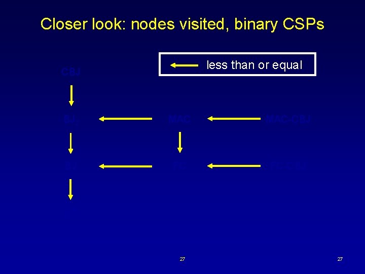
Closer look: nodes visited, binary CSPs less than or equal CBJ BJ 2 MAC-CBJ BJ FC FC-CBJ BT 27 27

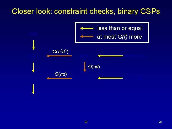
Closer look: constraint checks, binary CSPs less than or equal CBJ BJ 2 at most O(f) more O(n 2 d 2) MAC-CBJ O(nd) FC FC-CBJ BT 28 28

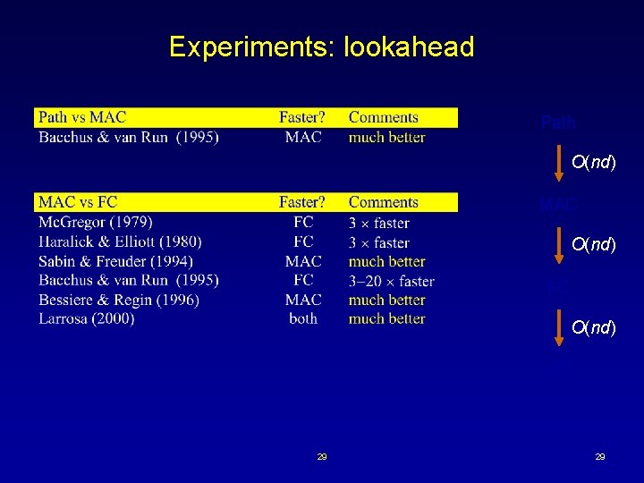
Experiments: lookahead Path O(nd) MAC O(nd) FC O(nd) BT 29 29

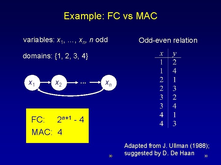
Example: FC vs MAC variables: x 1, …, xn, n odd Odd-even relation domains: {1, 2, 3, 4} x 1 x 2 . . . xn FC: 2 n+1 - 4 MAC: 4 30 Adapted from J. Ullman (1988); suggested by D. De Haan 30

Increasing lookahead Time (sec. ) to solve 6 x 6 puzzles MC 4 MC 3 MC 2 MC 1 31 31

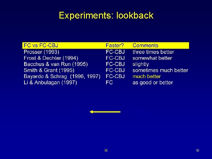
Experiments: lookback FC FC-CBJ 32 32

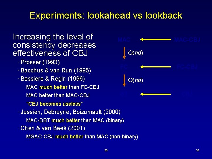
Experiments: lookahead vs lookback Increasing the level of consistency decreases effectiveness of CBJ MAC-CBJ O(nd) · Prosser (1993) · Bacchus & van Run (1995) · Bessiere & Regin (1996) FC FC-CBJ O(nd) MAC much better than FC-CBJ BT MAC better than MAC-CBJ “CBJ becomes useless” · Jussien, Debruyne, Boizumault (2000) MAC-DBT much better than MAC (binary) · Chen & van Beek (2001) MGAC-CBJ much better than MAC (non-binary) 33 33

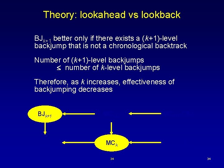
Theory: lookahead vs lookback BJk+1 better only if there exists a (k+1)-level backjump that is not a chronological backtrack Number of (k+1)-level backjumps number of k-level backjumps Therefore, as k increases, effectiveness of backjumping decreases BJk+1 MCk+1 -CBJ BJk MCk-CBJ 34 34

Part II Comparing CSP models 35 35

Conversion to binary Any non-binary CSP can be converted into one with only binary constraints ·dual graph method (Dechter & Pearl, 1989; Rossi et al. 1989) ·hidden variable method (Peirce, 1933; Rossi et al. 1989; Dechter 1990) 36 36

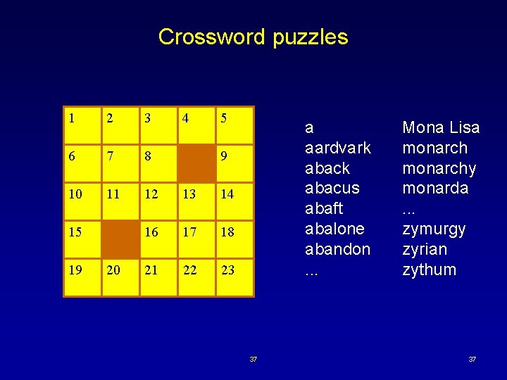
Crossword puzzles 1 2 3 6 7 8 10 11 12 13 14 16 17 18 21 22 23 15 19 20 4 5 a aardvark abacus abaft abalone abandon. . . 9 37 Mona Lisa monarchy monarda. . . zymurgy zyrian zythum 37

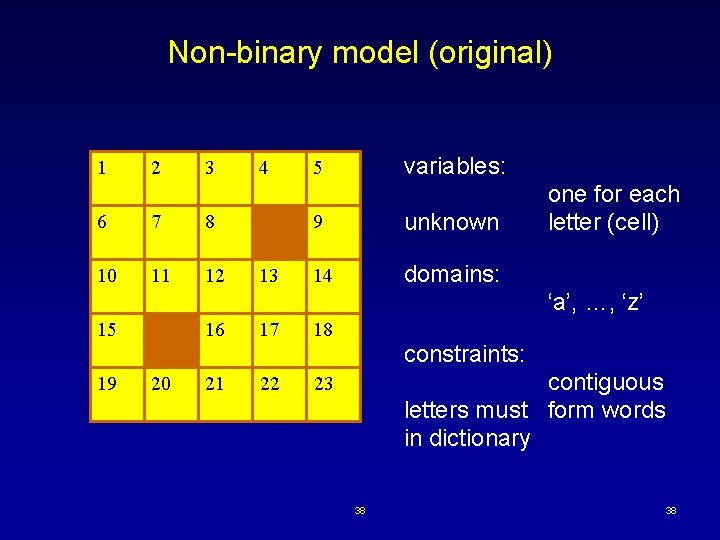
Non-binary model (original) 1 2 3 6 7 8 10 11 12 4 13 variables: 5 9 unknown 14 domains: one for each letter (cell) ‘a’, …, ‘z’ 15 16 17 18 constraints: 19 20 21 22 contiguous letters must form words in dictionary 23 38 38

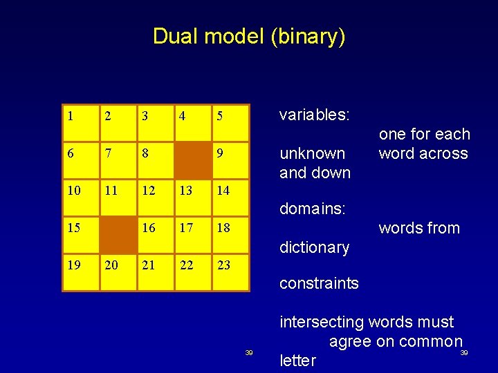
Dual model (binary) 1 2 3 6 7 8 10 11 12 4 variables: 5 unknown and down 9 13 one for each word across 14 domains: 15 16 17 words from 18 dictionary 19 20 21 22 23 constraints 39 intersecting words must agree on common 39 letter

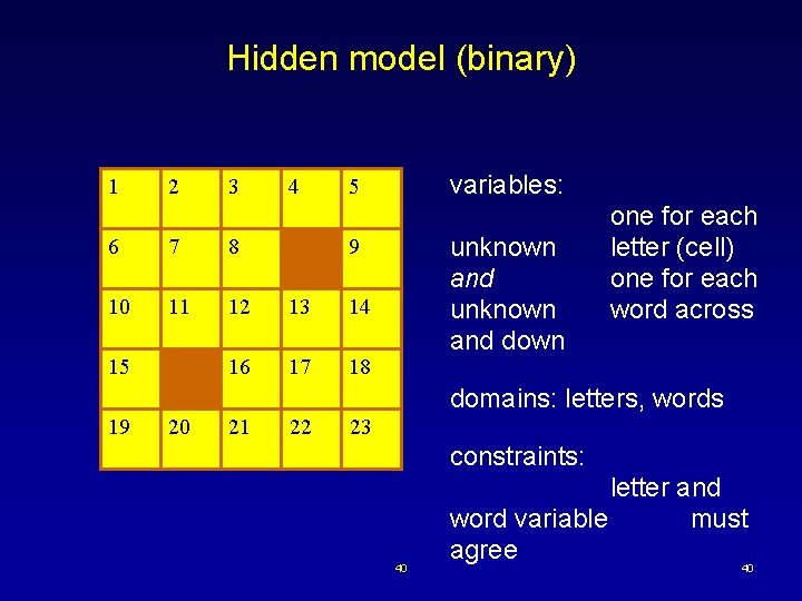
Hidden model (binary) 1 2 3 4 6 7 8 10 11 12 13 14 16 17 18 15 variables: 5 unknown and down 9 one for each letter (cell) one for each word across domains: letters, words 19 20 21 22 23 constraints: 40 letter and word variable must agree 40

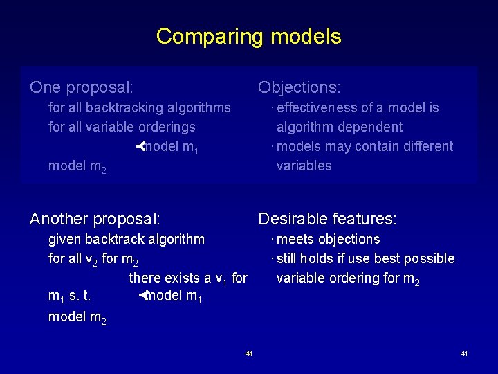
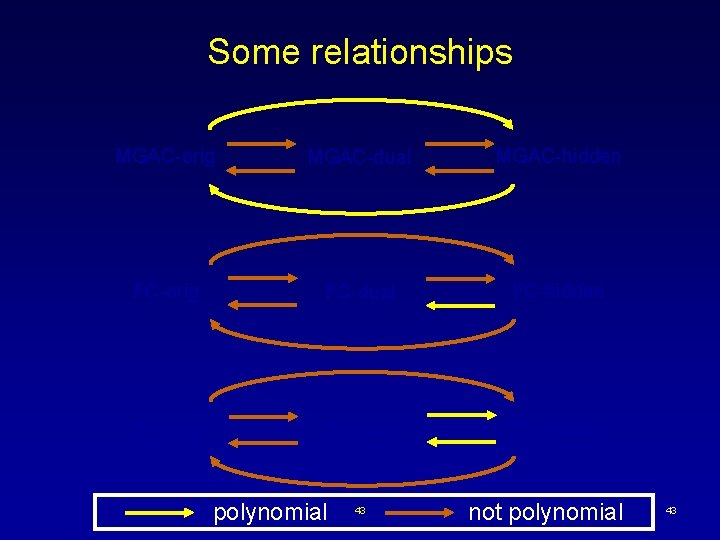
Comparing models One proposal: Objections: · effectiveness of a model is algorithm dependent · models may contain different variables for all backtracking algorithms for all variable orderings model m 1 model m 2 Another proposal: Desirable features: given backtrack algorithm for all v 2 for m 2 there exists a v 1 for m 1 s. t. model m 1 · meets objections · still holds if use best possible variable ordering for m 2 model m 2 41 41

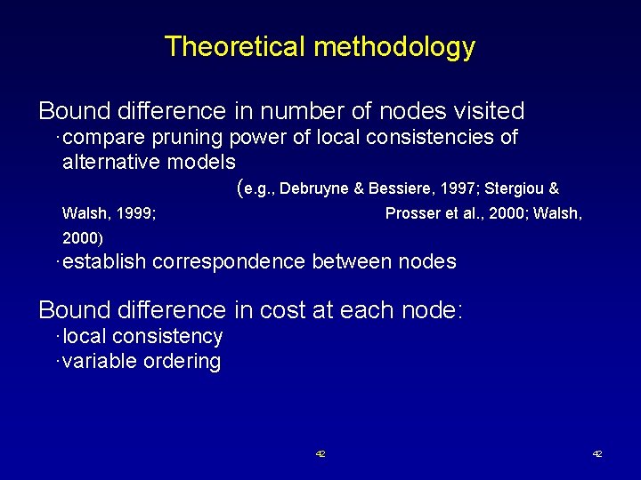
Theoretical methodology Bound difference in number of nodes visited ·compare pruning power of local consistencies of alternative models (e. g. , Debruyne & Bessiere, 1997; Stergiou & Walsh, 1999; Prosser et al. , 2000; Walsh, 2000) ·establish correspondence between nodes Bound difference in cost at each node: ·local consistency ·variable ordering 42 42

Some relationships MGAC-orig MGAC-dual MGAC-hidden FC-orig FC-dual FC-hidden BT-orig BT-dual BT-hidden polynomial 43 not polynomial 43

Part III Comparing variable ordering heuristics Future work 44 44

Conclusion Technical: ·comparing backtracking algorithms partial order ·comparing CSP models bounded worse relation on algorithm-model combinations Big picture: ·theory can guide, inform experimentation 45 45