Towards Efficient Sampling Exploiting Random Walk Strategy Wei

Towards Efficient Sampling: Exploiting Random Walk Strategy Wei, Jordan Erenrich, and Bart Selman 1

Motivations Recent years have seen tremendous improvements in SAT solving. Formulas with up to 300 variables (1992) to formulas with one million variables. n Various techniques for answering “does a satisfying assignment exist for a formula? ” n But there are harder questions to be answered. “how many satisfying assignments does a formula have? ” Or closely related “can we sample from the satisfying assignments of a formula? ” n 2

Complexity n SAT is NP-complete. 2 -SAT is solvable in linear time. n Counting assignments (even for 2 cnf) is #P-complete, and is NP-hard to approximate (Valiant, 1979). n Approximate counting and sampling are equivalent if the problem is “downward self-reducible”. 3

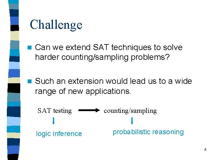
Challenge n Can we extend SAT techniques to solve harder counting/sampling problems? n Such an extension would lead us to a wide range of new applications. SAT testing logic inference counting/sampling probabilistic reasoning 4

Standard Methods for Sampling MCMC n Based on setting up a Markov chain with a predefined stationary distribution. n Draw samples from the stationary distribution by running the Markov chain for sufficiently long. n Problem: for interesting problems, Markov chain takes exponential time to converge to its stationary distribution 5

Simulated Annealing uses Boltzmann distribution as the stationary distribution. n At low temperature, the distribution concentrates around minimum energy states. n In terms of satisfiability problem, each satisfying assignment (with 0 cost) gets the same probability. n Again, reaching such a stationary distribution takes exponential time for interesting problems. – shown in a later slide. n 6

Standard Methods for Counting n Current solution counting procedures extend DPLL methods with component analysis. n Two counting precedures are available. relsat (Bayardo and Pehoushek, 2000) and cachet (Sang, Beame, and Kautz, 2004). They both count exact number of solutions. 7

n Question: Can state-of-the-art local search procedures be used for SAT sampling/counting? (as alternatives to standard Monte Carlo Markov Chain and DPLL methods) Yes! Shown in this talk 8

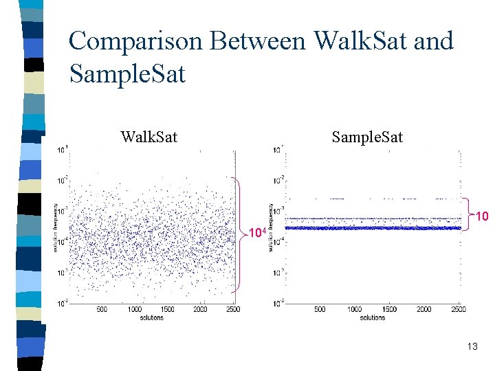
Our approach – biased random walk n Biased random walk = greedy bias + pure random walk. Example: Walk. Sat (Selman et al, 1994), effective on SAT. n Can we use it to sample from solution space? – Does Walk. Sat reach all solutions? – How uniform is the sampling? 9

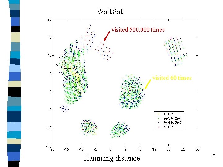
Walk. Sat visited 500, 000 times visited 60 times Hamming distance 10

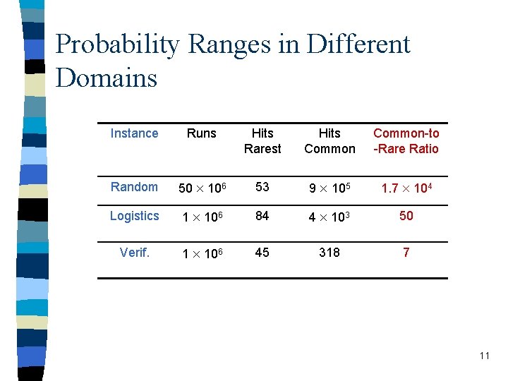
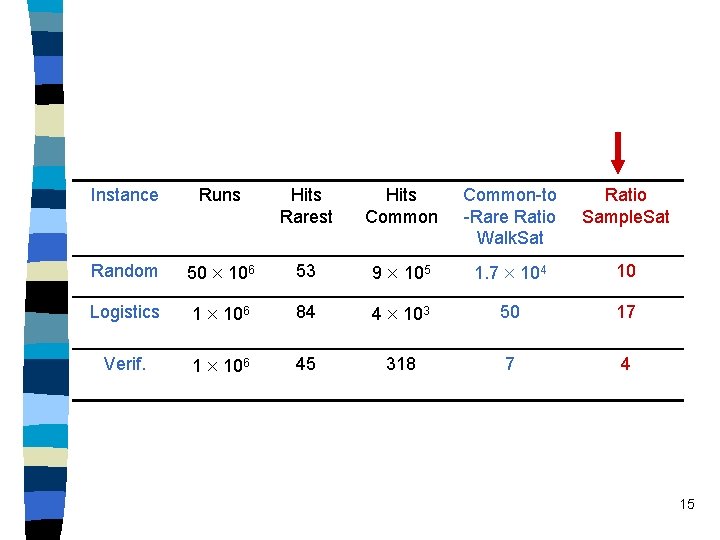
Probability Ranges in Different Domains Instance Runs Hits Rarest Hits Common-to -Rare Ratio Random 50 106 53 9 105 1. 7 104 Logistics 1 106 84 4 103 50 Verif. 1 106 45 318 7 11

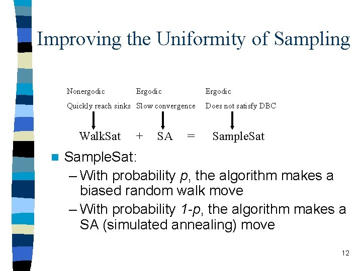
Improving the Uniformity of Sampling Nonergodic Ergodic Quickly reach sinks Slow convergence Walk. Sat n + SA = Does not satisfy DBC Sample. Sat: – With probability p, the algorithm makes a biased random walk move – With probability 1 -p, the algorithm makes a SA (simulated annealing) move 12

Comparison Between Walk. Sat and Sample. Sat Walk. Sat Sample. Sat 10 104 13

Sample. Sat Hamming Distance 14

Instance Runs Hits Rarest Hits Common-to -Rare Ratio Walk. Sat Ratio Sample. Sat Random 50 106 53 9 105 1. 7 104 10 Logistics 1 106 84 4 103 50 17 Verif. 1 106 45 318 7 4 15

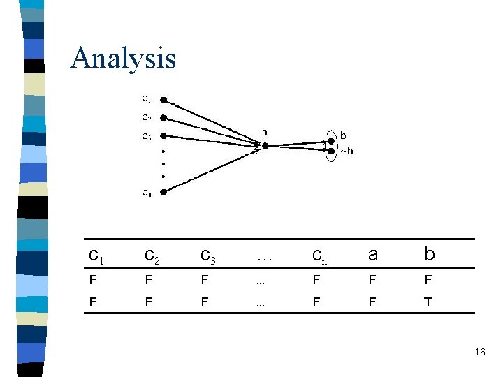
Analysis c 1 c 2 c 3 … cn a b F F F … F F T 16

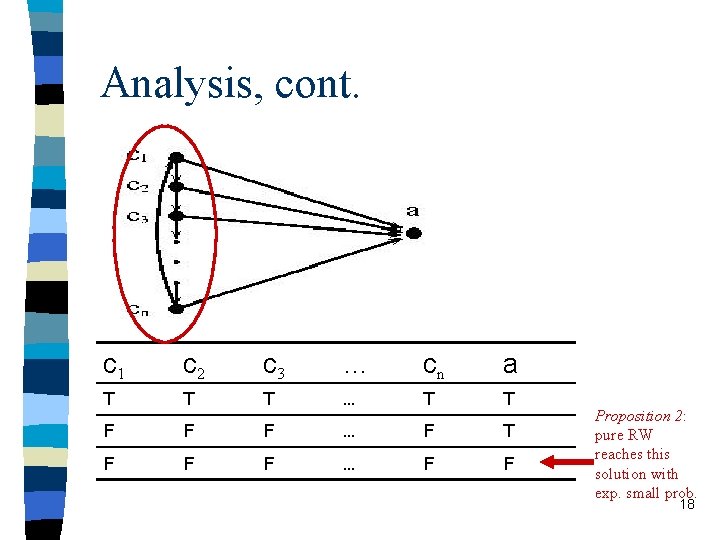
Property of F* n Proposition 1 SA with fixed temperature takes exponential time to find a solution of F* n This shows even for some simple formulas in 2 cnf, SA cannot reach a solution in poly-time 17

Analysis, cont. c 1 c 2 c 3 … cn a T T T … T T F F F … F F Proposition 2: pure RW reaches this solution with exp. small prob. 18

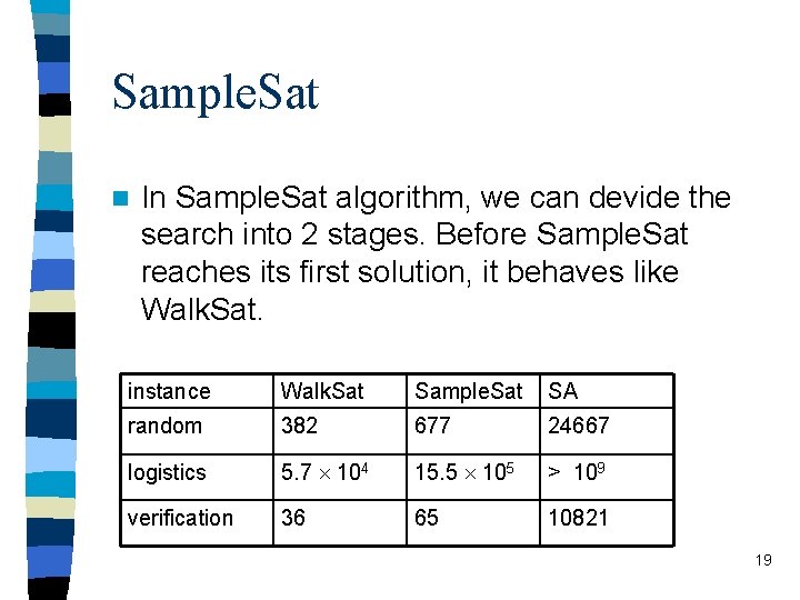
Sample. Sat n In Sample. Sat algorithm, we can devide the search into 2 stages. Before Sample. Sat reaches its first solution, it behaves like Walk. Sat. instance Walk. Sat Sample. Sat SA random 382 677 24667 logistics 5. 7 104 15. 5 105 > 109 verification 36 65 10821 19

Sample. Sat, cont. After reaching the solution, random walk component is turned off because all clauses are satisfied. Sample. Sat behaves like SA. n Proposition 3 SA at zero temperature samples all solutions within a cluster uniformly. n This 2 -stage model explains why Sample. Sat samples more uniformly than random walk algorithms alone. n 20

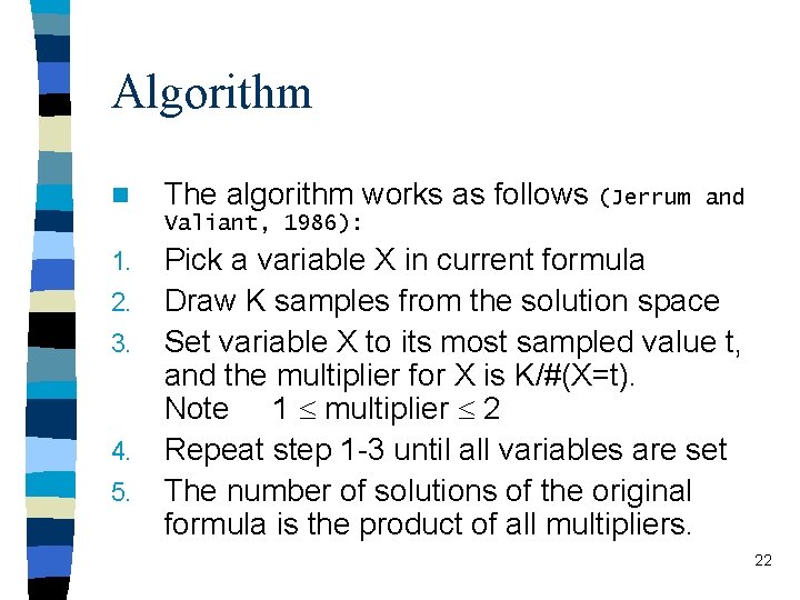
Verification on Larger formulas Approx. Count Small formulas -> Figures, solution frequencies. How to verify on large formulas? Approx. Count. n Approx. Count approximates the number of solutions of Boolean formulas, based on Sample. Sat algorithm. n Besides using it to justify the accuracy of our sampling approach, Approx. Count is interesting on its own right. n 21

Algorithm n The algorithm works as follows (Jerrum and Valiant, 1986): 1. 2. 3. 4. 5. Pick a variable X in current formula Draw K samples from the solution space Set variable X to its most sampled value t, and the multiplier for X is K/#(X=t). Note 1 multiplier 2 Repeat step 1 -3 until all variables are set The number of solutions of the original formula is the product of all multipliers. 22

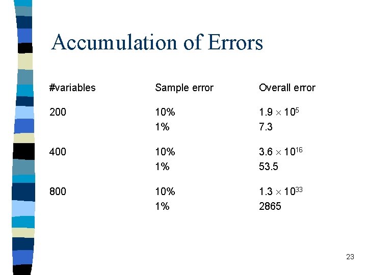
Accumulation of Errors #variables Sample error Overall error 200 10% 1% 1. 9 105 7. 3 400 10% 1% 3. 6 1016 53. 5 800 10% 1% 1. 3 1033 2865 23

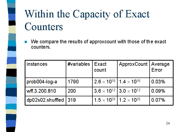
Within the Capacity of Exact Counters n We compare the results of approxcount with those of the exact counters. instances #variables Exact count Approx. Count Average Error prob 004 -log-a 1790 2. 6 1016 1. 4 1016 0. 03% wff. 3. 200. 810 200 3. 6 1012 3. 0 1012 0. 09% dp 02 s 02. shuffled 319 1. 5 1025 1. 2 1025 0. 07% 24

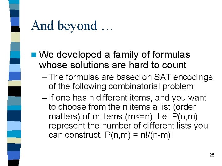
And beyond … n We developed a family of formulas whose solutions are hard to count – The formulas are based on SAT encodings of the following combinatorial problem – If one has n different items, and you want to choose from the n items a list (order matters) of m items (m<=n). Let P(n, m) represent the number of different lists you can construct. P(n, m) = n!/(n-m)! 25

Hard Instances Encoding of P(20, 10) has only 200 variables, but neither cachet or Relsat was able to count it in 5 days in our experiments. n On the other hard, Approx. Count is able to finish in 2 hours, and estimates the solutions of even larger instances. n instance #variables #solutions Approx. Count Average Error P(30, 20) 600 7 1025 7 1024 0. 4% P(20, 10) 200 7 1011 2 1011 0. 6% 26

Summary n Small formulas -> complete analysis of the search space n Larger formulas -> compare Approx. Count results with results of exact counting procedures n Harder formulas -> handcraft formulas compare with analytic results 27

Conclusion and Future Work n Shows good opportunity to extend SAT solvers to develop algorithms for sampling and counting tasks. n Next step: Use our methods in probabilistic reasoning and Bayesian inference domains. 28