Towards Dynamic GPCA Hybrid System Identification for the

Towards Dynamic GPCA Hybrid System Identification for the Analysis of Dynamic Scenes René Vidal Center for Imaging Science Johns Hopkins University

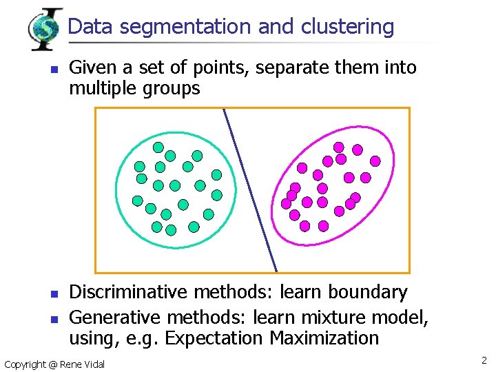
Data segmentation and clustering n n n Given a set of points, separate them into multiple groups Discriminative methods: learn boundary Generative methods: learn mixture model, using, e. g. Expectation Maximization Copyright @ Rene Vidal 2

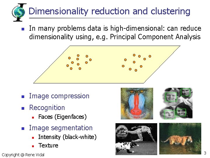
Dimensionality reduction and clustering n In many problems data is high-dimensional: can reduce dimensionality using, e. g. Principal Component Analysis n Image compression n Recognition n n Faces (Eigenfaces) Image segmentation n n Intensity (black-white) Texture Copyright @ Rene Vidal 3

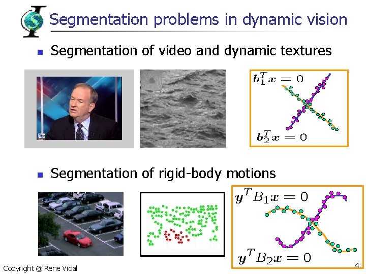
Segmentation problems in dynamic vision n Segmentation of video and dynamic textures n Segmentation of rigid-body motions Copyright @ Rene Vidal 4

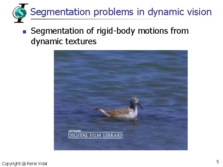
Segmentation problems in dynamic vision n Segmentation of rigid-body motions from dynamic textures Copyright @ Rene Vidal 5

Clustering data on non Euclidean spaces n n n n “Chicken-and-egg” problems n n Mixtures of linear spaces Mixtures of algebraic varieties Mixtures of Lie groups Given segmentation, estimate models Given models, segment the data Initialization? Need to combine n Algebra/geometry, dynamics and statistics Copyright @ Rene Vidal 6

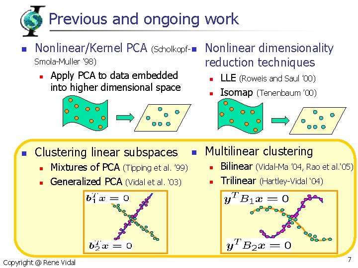
Previous and ongoing work n Nonlinear/Kernel PCA (Scholkopf- n Smola-Muller ’ 98) n n Apply PCA to data embedded into higher dimensional space Clustering linear subspaces n n Mixtures of PCA (Tipping et al. ’ 99) Generalized PCA (Vidal et al. ‘ 03) Copyright @ Rene Vidal Nonlinear dimensionality reduction techniques n n n LLE (Roweis and Saul ’ 00) Isomap (Tenenbaum ’ 00) Multilinear clustering n n Bilinear (Vidal-Ma ’ 04, Rao et al. ‘ 05) Trilinear (Hartley-Vidal ‘ 04) 7

Toward Dynamic GPCA n GPCA is a batch technique n Time series data is considered as a high-dimensional vector Time series data is projected onto low-dimensional space GPCA is applied to projected data as if they were static n Disadvantage of applying GPCA to time-series data n n n Does not model temporal evolution of the data It is not causal and cannot operate in real-time Dynamic GPCA n Model scene as mixture of dynamical models exhibiting changes n n n Space: multiple motions in the scene Time: appearing and disappearing objects “Try” to solve the identification problem using recursive identification techniques Copyright @ Rene Vidal 8

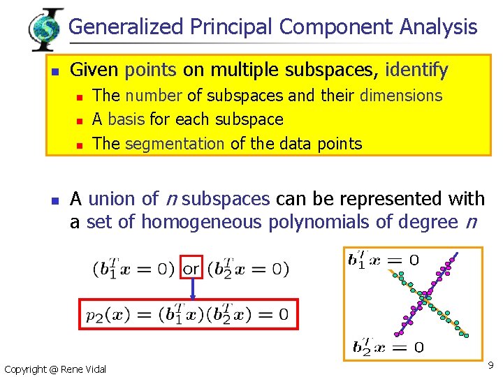
Generalized Principal Component Analysis n Given points on multiple subspaces, identify n n The number of subspaces and their dimensions A basis for each subspace The segmentation of the data points A union of n subspaces can be represented with a set of homogeneous polynomials of degree n Copyright @ Rene Vidal 9

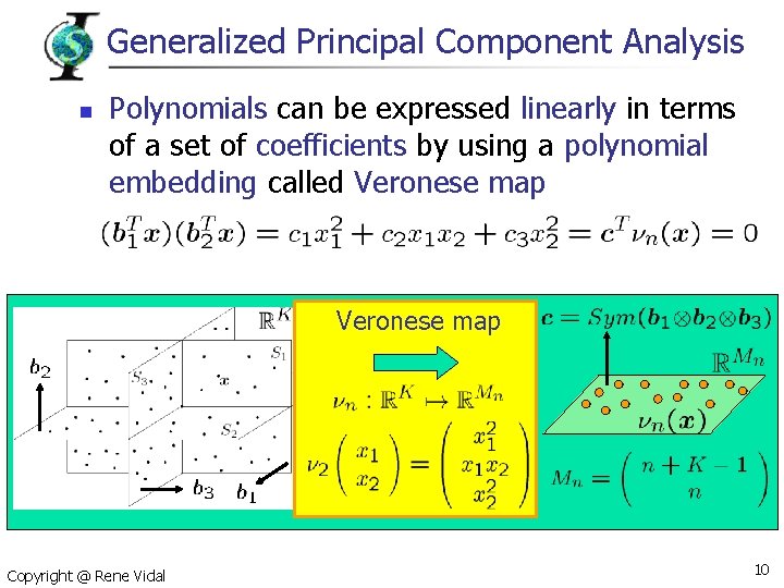
Generalized Principal Component Analysis n Polynomials can be expressed linearly in terms of a set of coefficients by using a polynomial embedding called Veronese map Copyright @ Rene Vidal 10

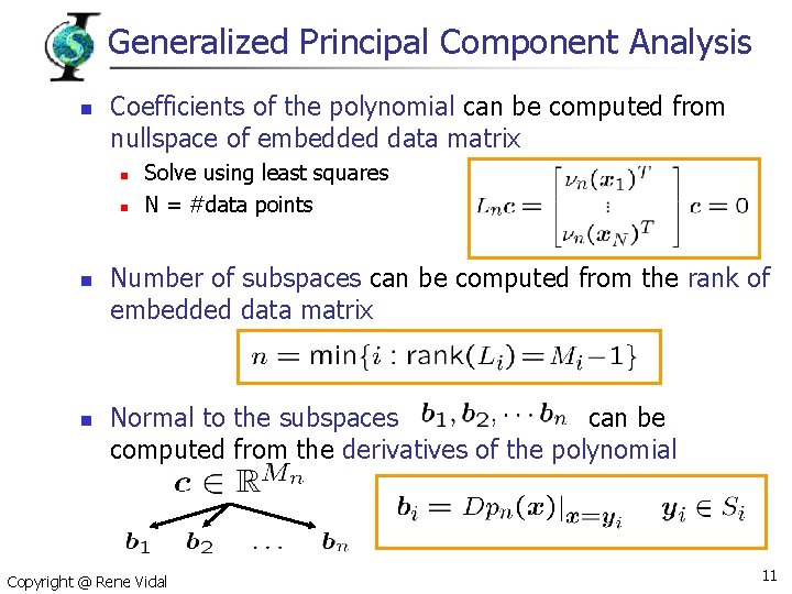
Generalized Principal Component Analysis n Coefficients of the polynomial can be computed from nullspace of embedded data matrix n n Solve using least squares N = #data points Number of subspaces can be computed from the rank of embedded data matrix Normal to the subspaces can be computed from the derivatives of the polynomial Copyright @ Rene Vidal 11

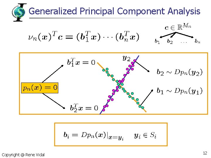
Generalized Principal Component Analysis Copyright @ Rene Vidal 12

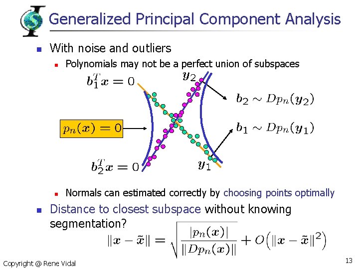
Generalized Principal Component Analysis n n With noise and outliers n Polynomials may not be a perfect union of subspaces n Normals can estimated correctly by choosing points optimally Distance to closest subspace without knowing segmentation? Copyright @ Rene Vidal 13

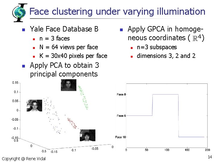
Face clustering under varying illumination n Yale Face Database B n n n = 3 faces N = 64 views per face K = 30 x 40 pixels per face n Apply GPCA in homogeneous coordinates ( ) n n n=3 subspaces dimensions 3, 2 and 2 Apply PCA to obtain 3 principal components Copyright @ Rene Vidal 14

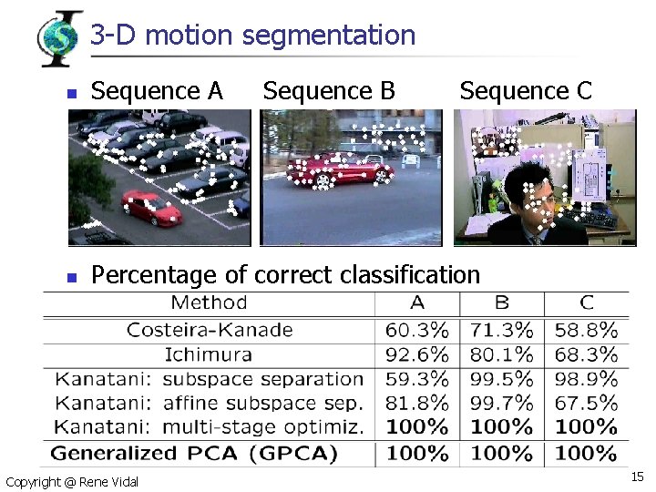
3 -D motion segmentation n Sequence A n Percentage of correct classification Copyright @ Rene Vidal Sequence B Sequence C 15

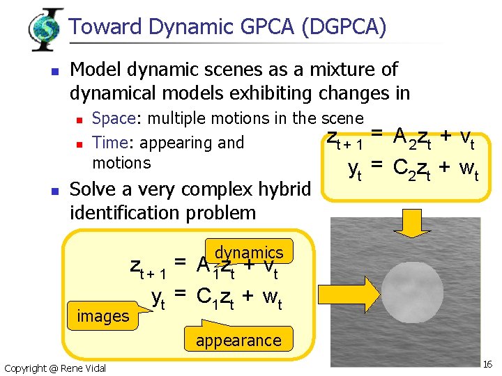
Toward Dynamic GPCA (DGPCA) n Model dynamic scenes as a mixture of dynamical models exhibiting changes in n Space: multiple motions in the scene zt + 1 Time: appearing and motions y Solve a very complex hybrid identification problem t = A z + vt disappearing 2 t = C 2 zt + wt system dynamics images zt + 1 = A 1 zt + vt yt = C 1 zt + wt appearance Copyright @ Rene Vidal 16

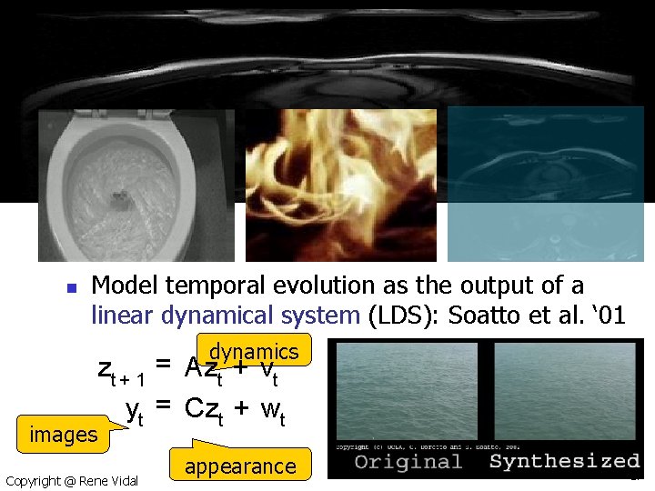
Modeling non-moving dynamic textures n n Examples of dynamic textures: Model temporal evolution as the output of a linear dynamical system (LDS): Soatto et al. ‘ 01 dynamics images zt + 1 = Azt + vt yt = Czt + wt Copyright @ Rene Vidal appearance 17

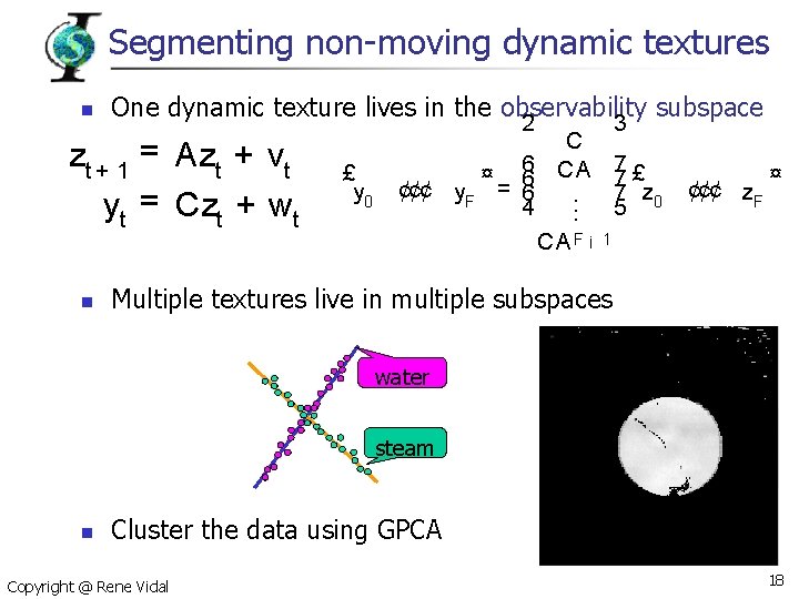
Segmenting non-moving dynamic textures n One dynamic texture lives in the observability subspace zt + 1 = Azt + vt yt = Czt + wt n 2 £ y 0 ¢¢¢ y. F ¤ 6 = 6 6 4 3 C CA. . . CA F ¡ 7£ 7 7 z 0 5 ¢¢¢ z. F ¤ 1 Multiple textures live in multiple subspaces water steam n Cluster the data using GPCA Copyright @ Rene Vidal 18

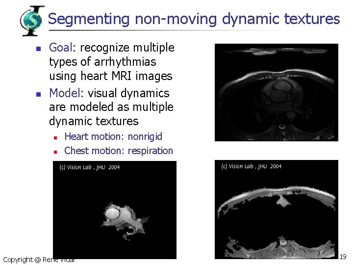
Segmenting non-moving dynamic textures n n Goal: recognize multiple types of arrhythmias using heart MRI images Model: visual dynamics are modeled as multiple dynamic textures n n Heart motion: nonrigid Chest motion: respiration Copyright @ Rene Vidal 19

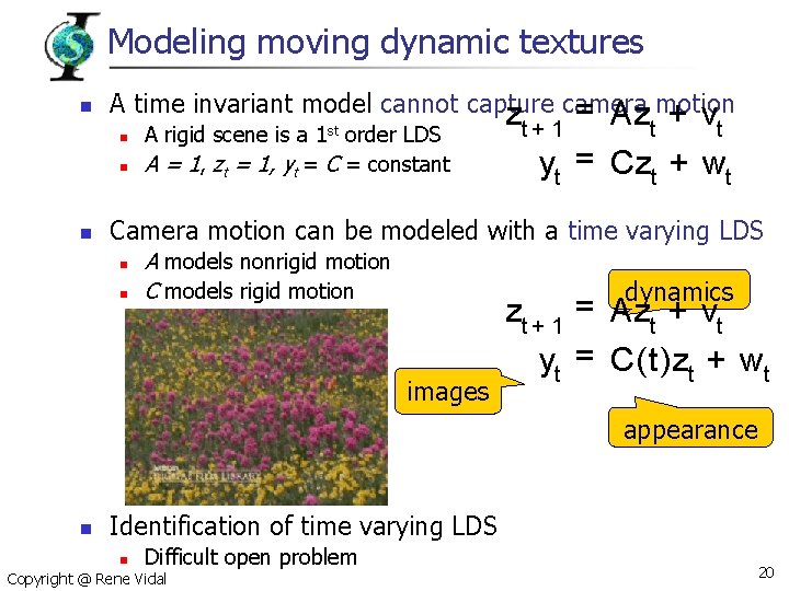
Modeling moving dynamic textures n A time invariant model cannot capture = Az motion z camera + v n n n A rigid scene is a 1 st order LDS A = 1, zt = 1, yt = C = constant t+ 1 t t yt = Czt + wt Camera motion can be modeled with a time varying LDS n n A models nonrigid motion C models rigid motion dynamics images zt + 1 = Azt + vt yt = C(t)zt + wt appearance n Identification of time varying LDS n Difficult open problem Copyright @ Rene Vidal 20

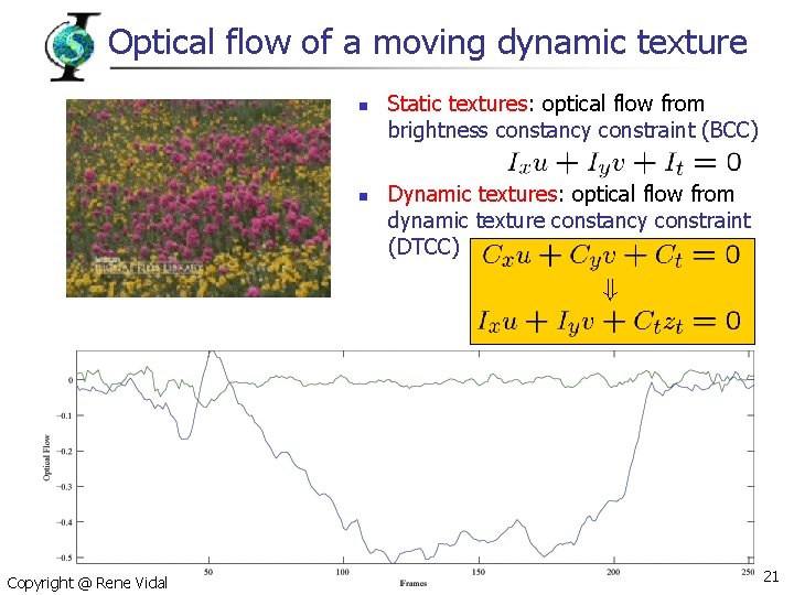
Optical flow of a moving dynamic texture n n Copyright @ Rene Vidal Static textures: optical flow from brightness constancy constraint (BCC) Dynamic textures: optical flow from dynamic texture constancy constraint (DTCC) 21

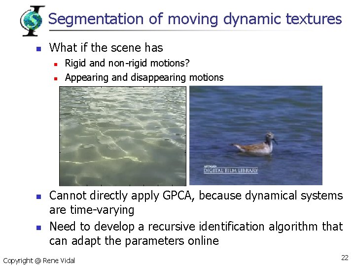
Segmentation of moving dynamic textures n What if the scene has n n Rigid and non-rigid motions? Appearing and disappearing motions Cannot directly apply GPCA, because dynamical systems are time-varying Need to develop a recursive identification algorithm that can adapt the parameters online Copyright @ Rene Vidal 22

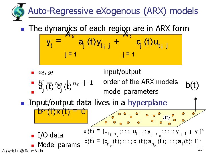
Auto-Regressive e. Xogenous (ARX) models n The dynamics of each region are in ARX form yt = Xn a aj (t)yt ¡ j j=1 n n aj (t); cj (t) + Xn c cj (t)ut ¡ j j=1 input/output order of the ARX models model parameters b(t) Input/output data lives in a hyperplane b> (t)x (t) = 0 n x (t) = [ut ¡ n c ; : : : ; u t ¡ 1 ; yt ¡ n a ; : : : ; yt ¡ 1 ; ¡ yt ]> I/O data b(t) = [cn (t); : : : ; c 1 (t); an (t); : : : ; a 1 (t); 1]> c a Model params 23 n Copyright @ Rene Vidal

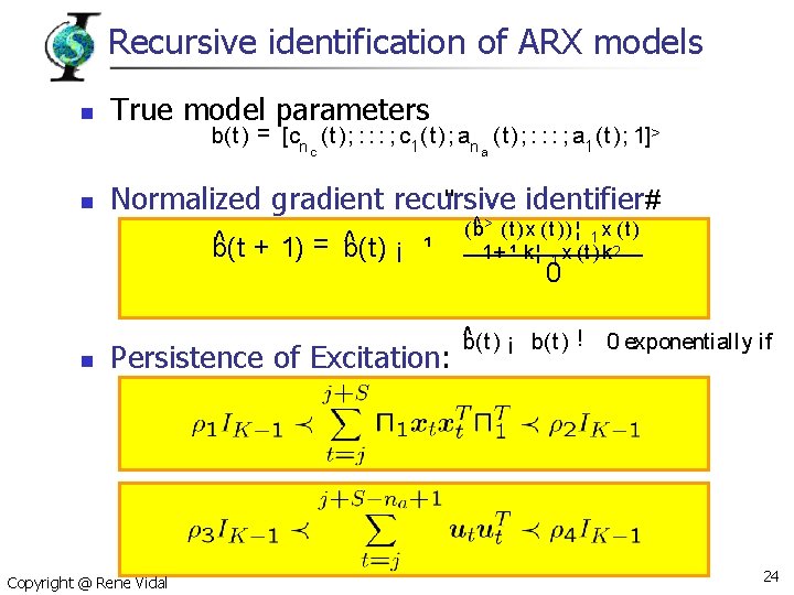
Recursive identification of ARX models n True model parameters b(t) = [cn (t); : : : ; c 1 (t); an (t); : : : ; a 1 (t); 1]> c n Normalized gradient recursive identifier# " ^ + 1) = b(t) ^ ¡ ¹ b(t n a Persistence of Excitation: Copyright @ Rene Vidal ^ > (t ) x ( t ) ) ¦ x ( t ) (b 1 1+ ¹ k¦ 1 x ( t ) k 2 0 ^ ¡ b(t) ! b(t) 0 exponentially if 24

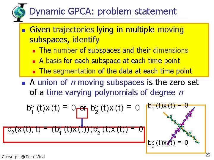
Dynamic GPCA: problem statement n Given trajectories lying in multiple moving subspaces, identify n n The number of subspaces and their dimensions A basis for each subspace at each time point The segmentation of the data at each time point A union of n moving subspaces is the zero set of a time varying polynomials of degree n b>1 (t)x (t) = 0 or b>2 (t)x (t) = 0 b>1 (t)x (t) = 0 p 2 (x (t); t) = (b>1 (t)x (t))(b>2 (t)x (t)) = 0 b>2 (t)x (t) = 0 Copyright @ Rene Vidal 25

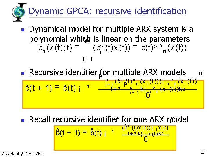
Dynamic GPCA: recursive identification n Dynamical model for multiple ARX system is a polynomial which Yn is linear on the parameters (b>i (t)x (t)) = c(t) > º n (x (t)) pn (x (t); t) = i= 1 n Recursive identifier " Pfor multiple ARX models c^ (t + 1) = c^ (t) ¡ ¹ n P ( c^ > ( t ) º n = i 1 P P 1+ ¹ i= 1 (x i ( t ) ) )¦ n º n ( x i ( t ) ) k¦ n º n ( x i (t ) )k 2 # 0 Recall recursive identifier" for one ARX model # ^ + 1) = b(t) ^ ¡ ¹ b(t Copyright @ Rene Vidal ^ > (t ) x ( t ) ) ¦ x ( t ) (b 1 1+ ¹ k¦ 1 x ( t ) k 2 0 26

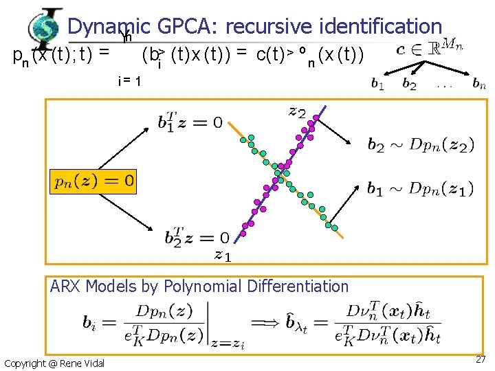
Dynamic GPCA: recursive identification Yn pn (x (t); t) = (b>i (t)x (t)) = c(t) > º n (x (t)) i= 1 ARX Models by Polynomial Differentiation Copyright @ Rene Vidal 27

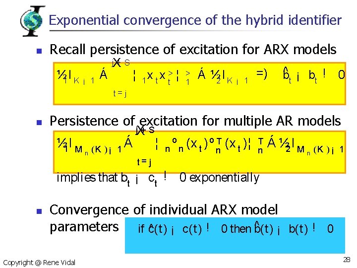
Exponential convergence of the hybrid identifier n Recall persistence of excitation for ARX models ½ 1 I K ¡ 1 Á j. X+ S ¦ 1 x t> ¦ > 1 Á ½ 2 I K ¡ 1 =) ^ ¡ b ! 0 b t t t= j n Persistence of excitation for multiple AR models ½ 1 I M n (K )¡ Á 1 j. X+ S ¦ T (x )¦ (x )º º t t n n n t= j implies that b c t ¡ ct ! n T n Á ½ 2 I M n (K )¡ 1 0 exponentially Convergence of individual ARX model ^ ¡ b(t) ! 0 parameters if c^ (t) ¡ c(t) ! 0 then b(t) Copyright @ Rene Vidal 28

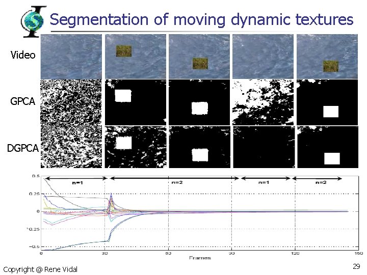
Segmentation of moving dynamic textures Video GPCA DGPCA Copyright @ Rene Vidal 29

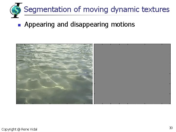
Segmentation of moving dynamic textures n Appearing and disappearing motions Copyright @ Rene Vidal 30

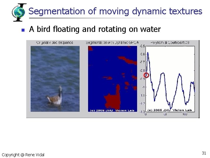
Segmentation of moving dynamic textures n A bird floating and rotating on water Copyright @ Rene Vidal 31

Summary n Many problems in computer vision can be posed as hybrid system identification problems n n n These problems can be solved using GPCA: an algorithm for clustering subspaces n n n Temporal video segmentation 2 -D and 3 -D motion segmentation Dynamic texture segmentation Nonrigid motion segmentation Deals with unknown and possibly different dimensions Deals with arbitrary intersections among the subspaces GPCA is based on n Projecting data onto a low-dimensional subspace Recursively fitting polynomials to projected subspaces Differentiating polynomials to obtain a basis Copyright @ Rene Vidal 32

Thanks n Johns Hopkins University n n Le Lu Avinash Ravichandran Dheeraj Singaraju n n n University of Illinois n n Yi Ma UCLA Stefano Soatto Australian National University Université des Sciences et Technologies de Lille n n Richard Hartley Camille Izard Università di Siena n Jacopo Piazzi UC Berkeley n Shankar Sastry Copyright @ Rene Vidal 33

Thanks n n n 2005 NSF CAREER "Recognition of Dynamic Activities in Unstructured Environments" 2005 NSF "An Algebraic Geometric Approach to Hybrid Systems Identification“ 2005 ONR “Segmenting Rigid Motions from Dynamic Textures” 2005 JHU “Advanced Video Exploitation for Unmanned Aerial Vehicles” 2004 NIH “Magnetic Resonance Guided Electrophysiology Intervention” Copyright @ Rene Vidal 34