Towards Decrypting the Art of Analog Layout Placement

Towards Decrypting the Art of Analog Layout: Placement Quality Prediction via Transfer Learning Mingjie Liu*, Keren Zhu*, Jiaqi Gu, Linxiao Shen, Xiyuan Tang, Nan Sun, and David Z. Pan Dept. of Electrical and Computer Engineering The University of Texas at Austin * Indicates equal contributions. 1

Outline Introduction and Motivation UT-An. Lay Dataset with MAGICAL Placement Quality Prediction Improved Data Efficiency with Transfer Learning Conclusions 2

Outline Introduction and Motivation UT-An. Lay Dataset with MAGICAL Placement Quality Prediction Improved Data Efficiency with Transfer Learning Conclusions 3

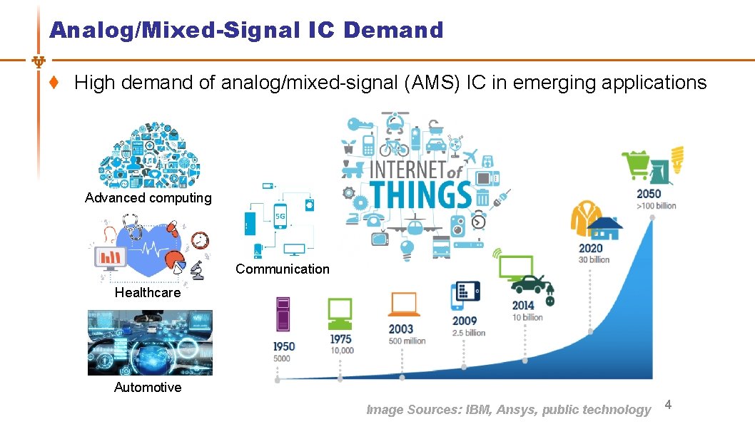
Analog/Mixed-Signal IC Demand High demand of analog/mixed-signal (AMS) IC in emerging applications Advanced computing Communication Healthcare Automotive Image Sources: IBM, Ansys, public technology 4

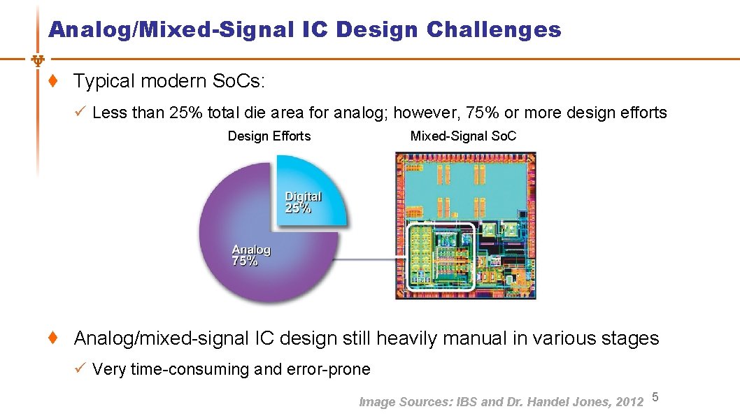
Analog/Mixed-Signal IC Design Challenges Typical modern So. Cs: ü Less than 25% total die area for analog; however, 75% or more design efforts Design Efforts Mixed-Signal So. C Analog/mixed-signal IC design still heavily manual in various stages ü Very time-consuming and error-prone Image Sources: IBS and Dr. Handel Jones, 2012 5

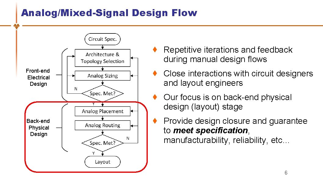
Analog/Mixed-Signal Design Flow Repetitive iterations and feedback during manual design flows Front-end Electrical Design Close interactions with circuit designers and layout engineers Our focus is on back-end physical design (layout) stage Back-end Physical Design Provide design closure and guarantee to meet specification, manufacturability, reliability, etc… 6

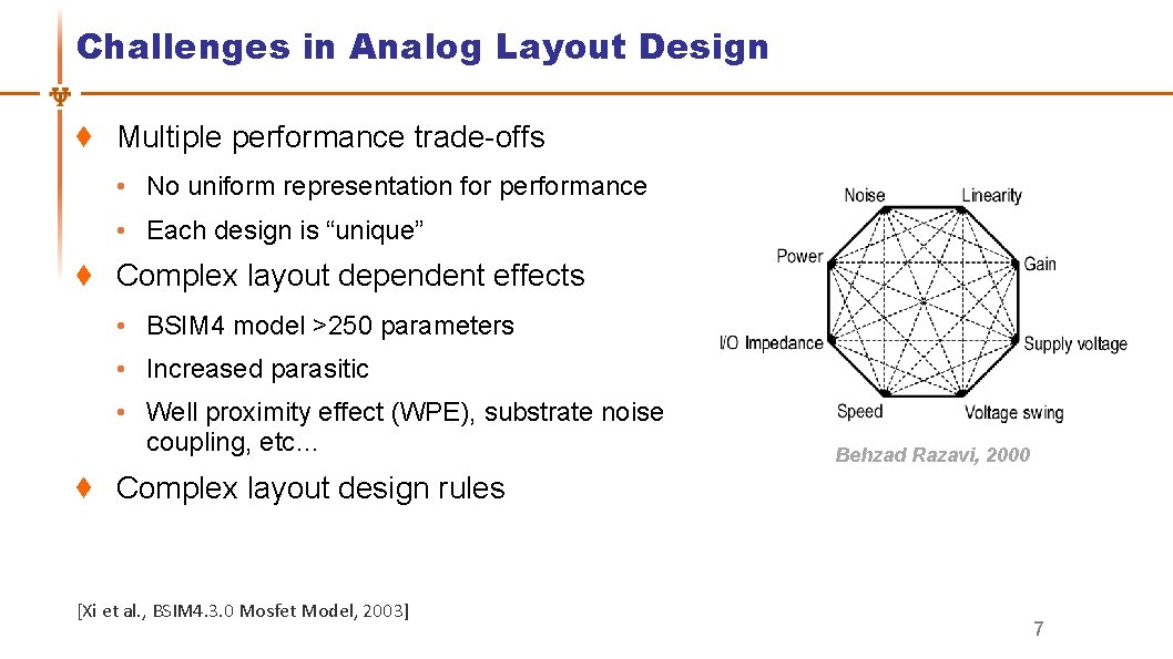
Challenges in Analog Layout Design Multiple performance trade-offs • No uniform representation for performance • Each design is “unique” Complex layout dependent effects • BSIM 4 model >250 parameters • Increased parasitic • Well proximity effect (WPE), substrate noise coupling, etc… Behzad Razavi, 2000 Complex layout design rules [Xi et al. , BSIM 4. 3. 0 Mosfet Model, 2003] 7

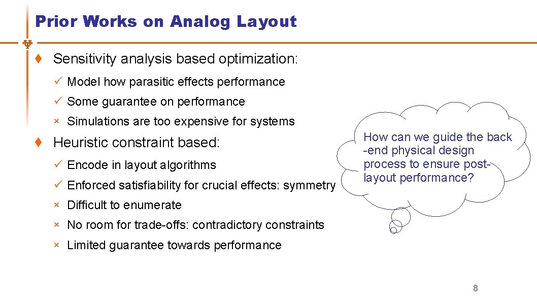
Prior Works on Analog Layout Sensitivity analysis based optimization: ü Model how parasitic effects performance ü Some guarantee on performance × Simulations are too expensive for systems Heuristic constraint based: ü Encode in layout algorithms ü Enforced satisfiability for crucial effects: symmetry How can we guide the back -end physical design process to ensure postlayout performance? × Difficult to enumerate × No room for trade-offs: contradictory constraints × Limited guarantee towards performance 8

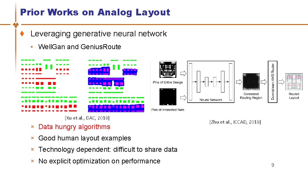
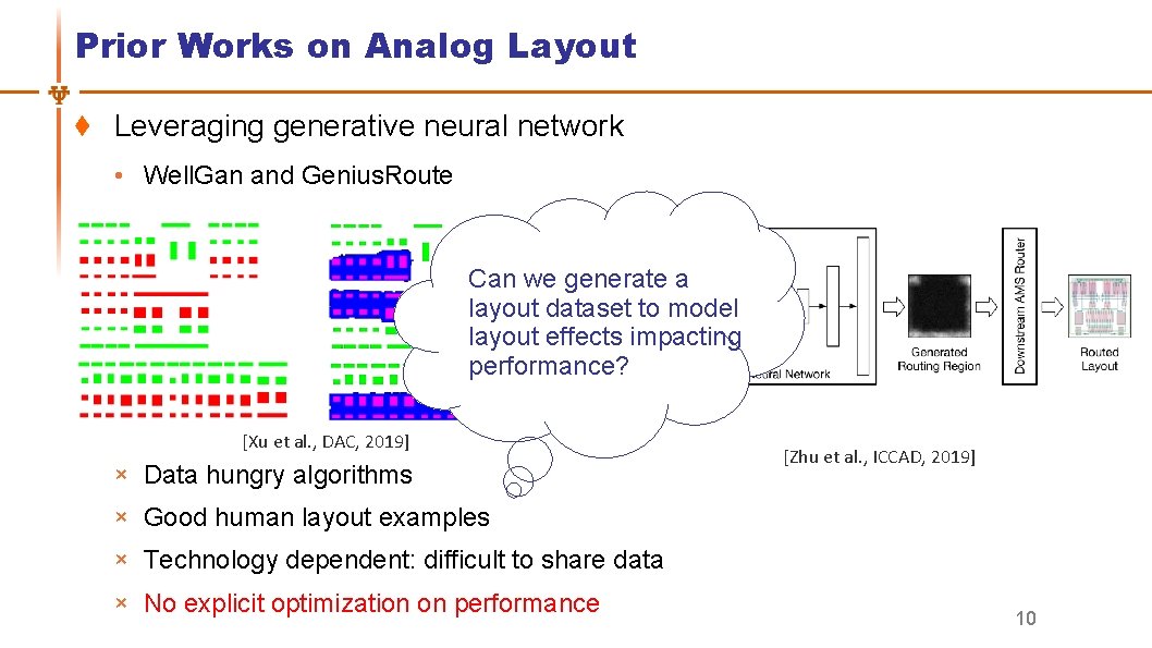
Prior Works on Analog Layout Leveraging generative neural network • Well. Gan and Genius. Route [Xu et al. , DAC, 2019] × Data hungry algorithms [Zhu et al. , ICCAD, 2019] × Good human layout examples × Technology dependent: difficult to share data × No explicit optimization on performance 9

Prior Works on Analog Layout Leveraging generative neural network • Well. Gan and Genius. Route Can we generate a layout dataset to model layout effects impacting performance? [Xu et al. , DAC, 2019] × Data hungry algorithms [Zhu et al. , ICCAD, 2019] × Good human layout examples × Technology dependent: difficult to share data × No explicit optimization on performance 10

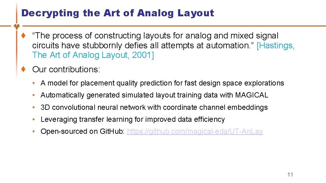
Decrypting the Art of Analog Layout “The process of constructing layouts for analog and mixed signal circuits have stubbornly defies all attempts at automation. ” [Hastings, The Art of Analog Layout, 2001] Our contributions: • A model for placement quality prediction for fast design space explorations • Automatically generated simulated layout training data with MAGICAL • 3 D convolutional neural network with coordinate channel embeddings • Leveraging transfer learning for improved data efficiency • Open-sourced on Git. Hub: https: //github. com/magical-eda/UT-An. Lay 11

Outline Introduction and Motivation UT-An. Lay Dataset with MAGICAL Placement Quality Prediction Improved Data Efficiency with Transfer Learning Conclusions 12

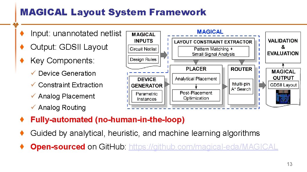
MAGICAL Layout System Framework Input: unannotated netlist Output: GDSII Layout Key Components: ü Device Generation ü Constraint Extraction ü Analog Placement ü Analog Routing Fully-automated (no-human-in-the-loop) Guided by analytical, heuristic, and machine learning algorithms Open-sourced on Git. Hub: https: //github. com/magical-eda/MAGICAL 13

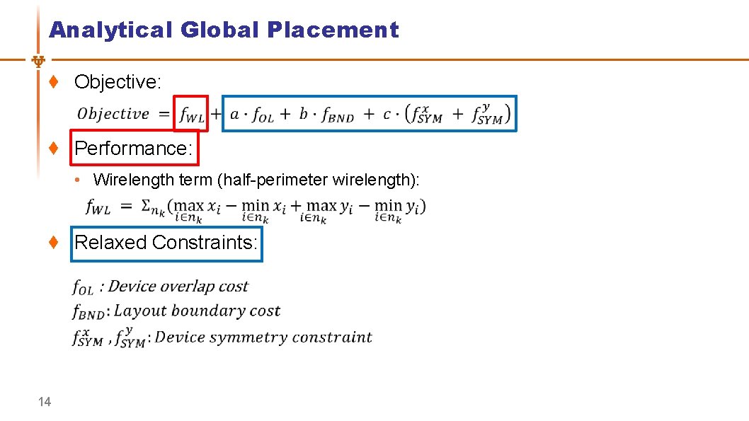
Analytical Global Placement Objective: Performance: • Wirelength term (half-perimeter wirelength): Relaxed Constraints: 14

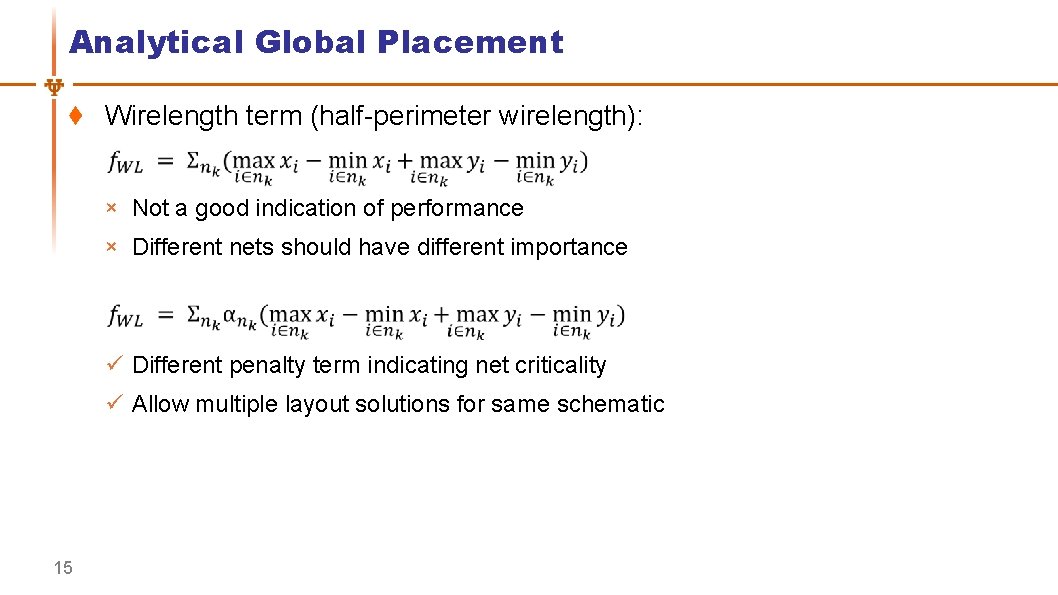
Analytical Global Placement Wirelength term (half-perimeter wirelength): × Not a good indication of performance × Different nets should have different importance ü Different penalty term indicating net criticality ü Allow multiple layout solutions for same schematic 15

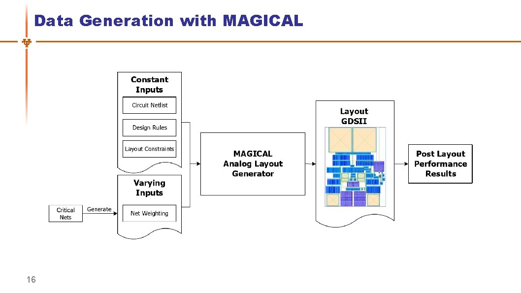
Data Generation with MAGICAL 16

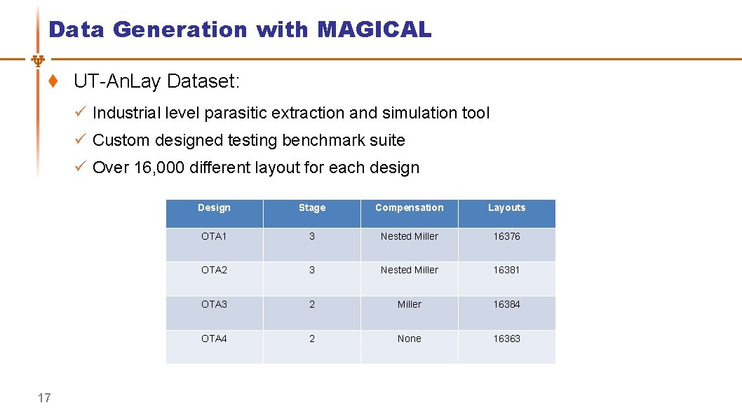
Data Generation with MAGICAL UT-An. Lay Dataset: ü Industrial level parasitic extraction and simulation tool ü Custom designed testing benchmark suite ü Over 16, 000 different layout for each design 17 Design Stage Compensation Layouts OTA 1 3 Nested Miller 16376 OTA 2 3 Nested Miller 16381 OTA 3 2 Miller 16384 OTA 4 2 None 16363

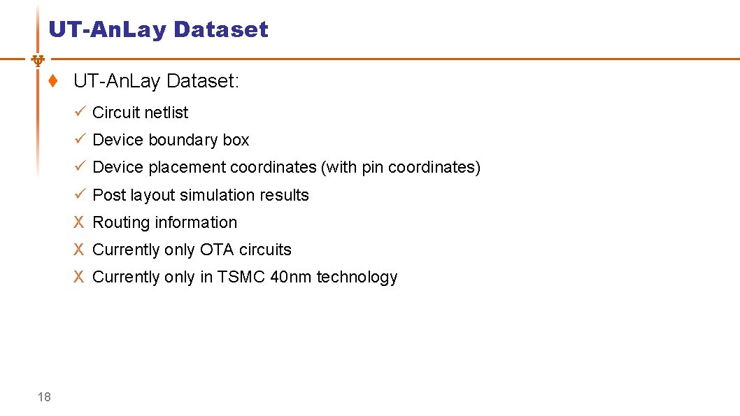
UT-An. Lay Dataset: ü Circuit netlist ü Device boundary box ü Device placement coordinates (with pin coordinates) ü Post layout simulation results X Routing information X Currently only OTA circuits X Currently only in TSMC 40 nm technology 18

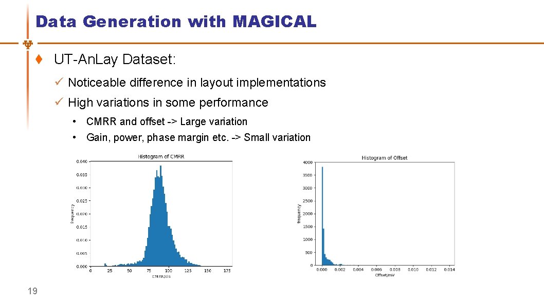
Data Generation with MAGICAL UT-An. Lay Dataset: ü Noticeable difference in layout implementations ü High variations in some performance • CMRR and offset -> Large variation • Gain, power, phase margin etc. -> Small variation 19

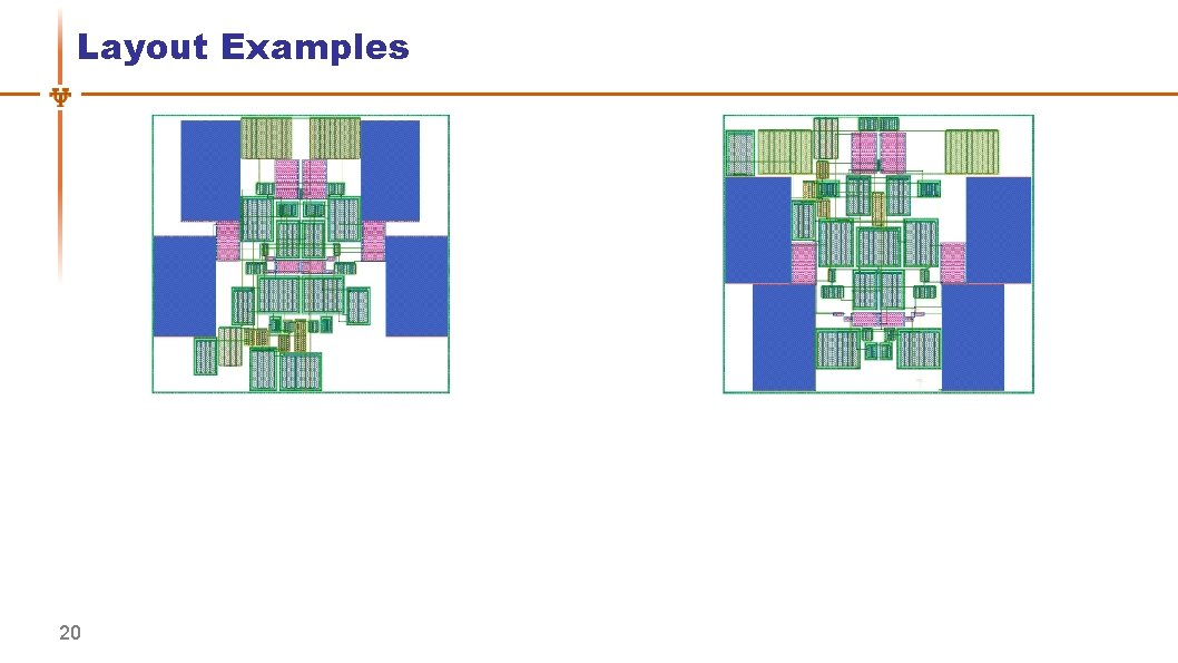
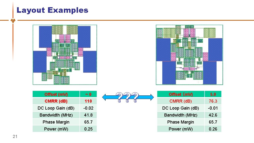
Layout Examples 20

Layout Examples 21 Offset (m. V) ~0 CMRR (d. B) 110 DC Loop Gain (d. B) ? ? ? Offset （m. V) 5. 0 CMRR (d. B) 76. 3 -0. 02 DC Loop Gain (d. B) -0. 01 Bandwidth (MHz) 41. 8 Bandwidth (MHz) 42. 6 Phase Margin 65. 7 Power (m. W) 0. 25 Power (m. W) 0. 26

Outline Introduction and Motivation UT-An. Lay Dataset with MAGICAL Placement Quality Prediction Improved Data Efficiency with Transfer Learning Conclusions 22

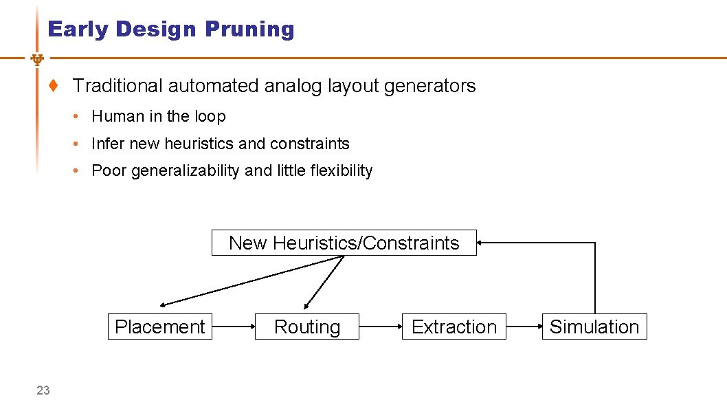
Early Design Pruning Traditional automated analog layout generators • Human in the loop • Infer new heuristics and constraints • Poor generalizability and little flexibility New Heuristics/Constraints Placement 23 Routing Extraction Simulation

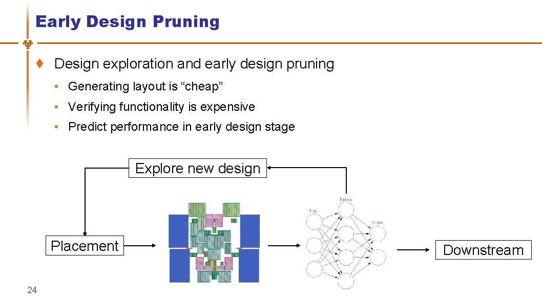
Early Design Pruning Design exploration and early design pruning • Generating layout is “cheap” • Verifying functionality is expensive • Predict performance in early design stage Explore new design Placement 24 Downstream

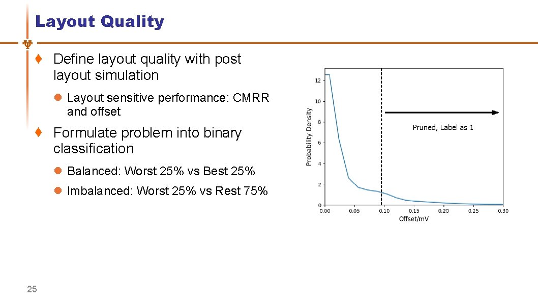
Layout Quality Define layout quality with post layout simulation l Layout sensitive performance: CMRR and offset Formulate problem into binary classification l Balanced: Worst 25% vs Best 25% l Imbalanced: Worst 25% vs Rest 75% 25

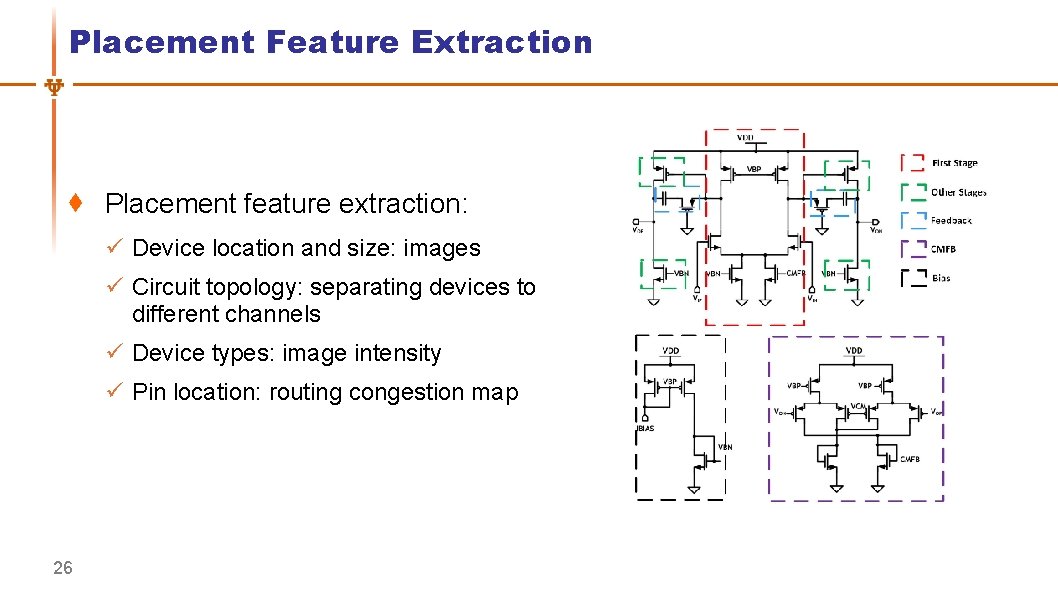
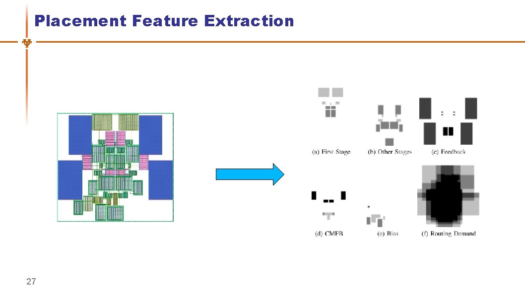
Placement Feature Extraction Placement feature extraction: ü Device location and size: images ü Circuit topology: separating devices to different channels ü Device types: image intensity ü Pin location: routing congestion map 26

Placement Feature Extraction 27

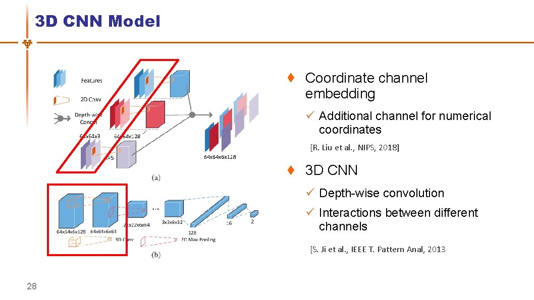
3 D CNN Model Coordinate channel embedding ü Additional channel for numerical coordinates [R. Liu et al. , NIPS, 2018] 3 D CNN ü Depth-wise convolution ü Interactions between different channels [S. Ji et al. , IEEE T. Pattern Anal, 2013 28

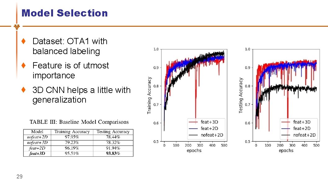
Model Selection Dataset: OTA 1 with balanced labeling Feature is of utmost importance 3 D CNN helps a little with generalization 29

Outline Introduction and Motivation UT-An. Lay Dataset with MAGICAL Placement Quality Prediction Improved Data Efficiency with Transfer Learning Conclusions 30

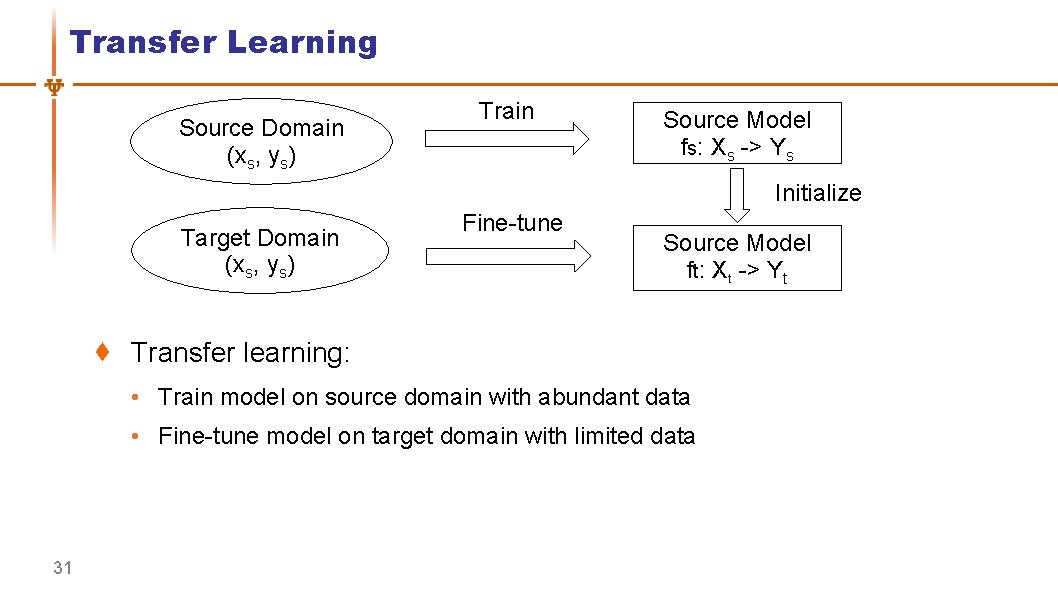
Transfer Learning Source Domain (xs, ys) Train Source Model fs: Xs -> Ys Initialize Target Domain (xs, ys) Fine-tune Source Model ft: Xt -> Yt Transfer learning: • Train model on source domain with abundant data • Fine-tune model on target domain with limited data 31

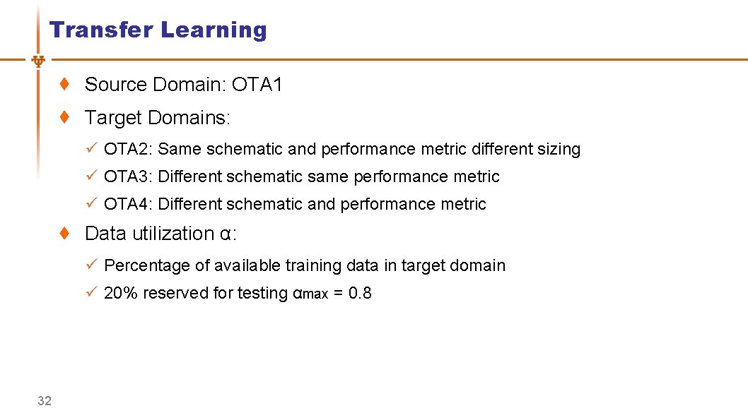
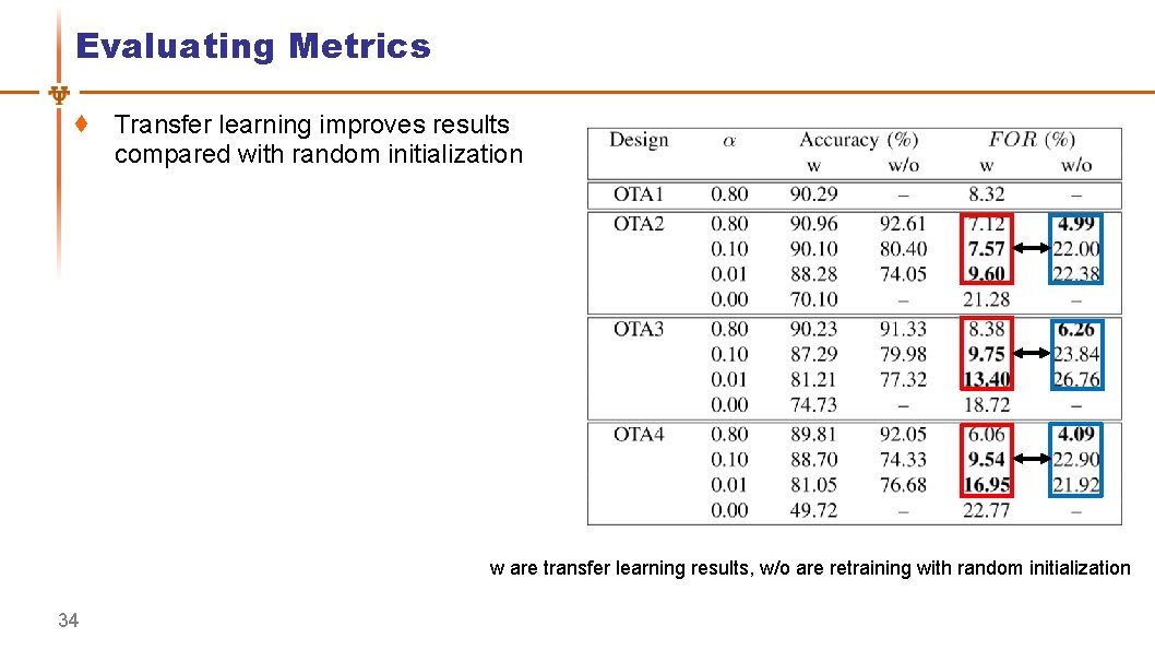
Transfer Learning Source Domain: OTA 1 Target Domains: ü OTA 2: Same schematic and performance metric different sizing ü OTA 3: Different schematic same performance metric ü OTA 4: Different schematic and performance metric Data utilization α: ü Percentage of available training data in target domain ü 20% reserved for testing αmax = 0. 8 32

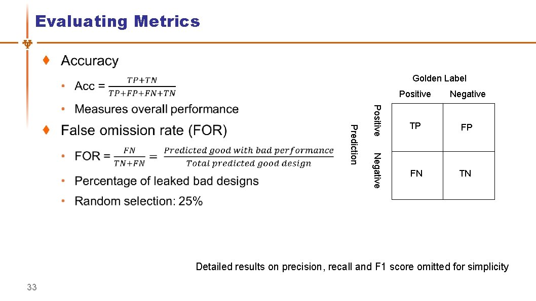
Evaluating Metrics Golden Label Positive Negative Prediction Positive Negative TP FP FN TN Detailed results on precision, recall and F 1 score omitted for simplicity 33

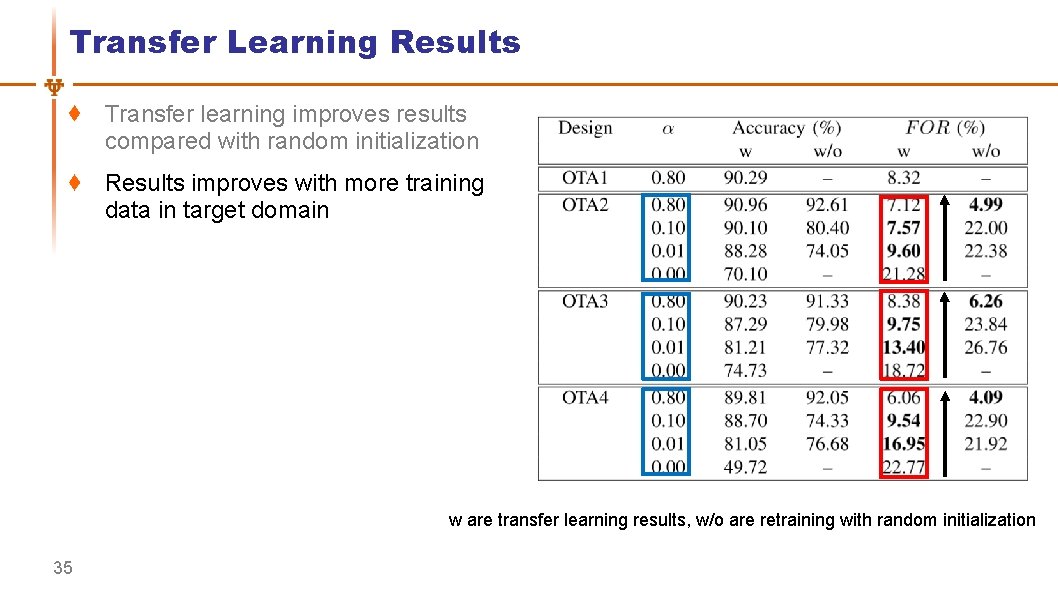
Evaluating Metrics Transfer learning improves results compared with random initialization w are transfer learning results, w/o are retraining with random initialization 34

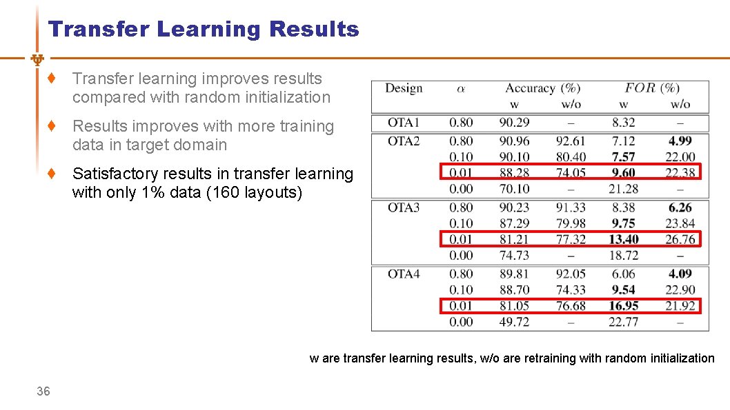
Transfer Learning Results Transfer learning improves results compared with random initialization Results improves with more training data in target domain w are transfer learning results, w/o are retraining with random initialization 35

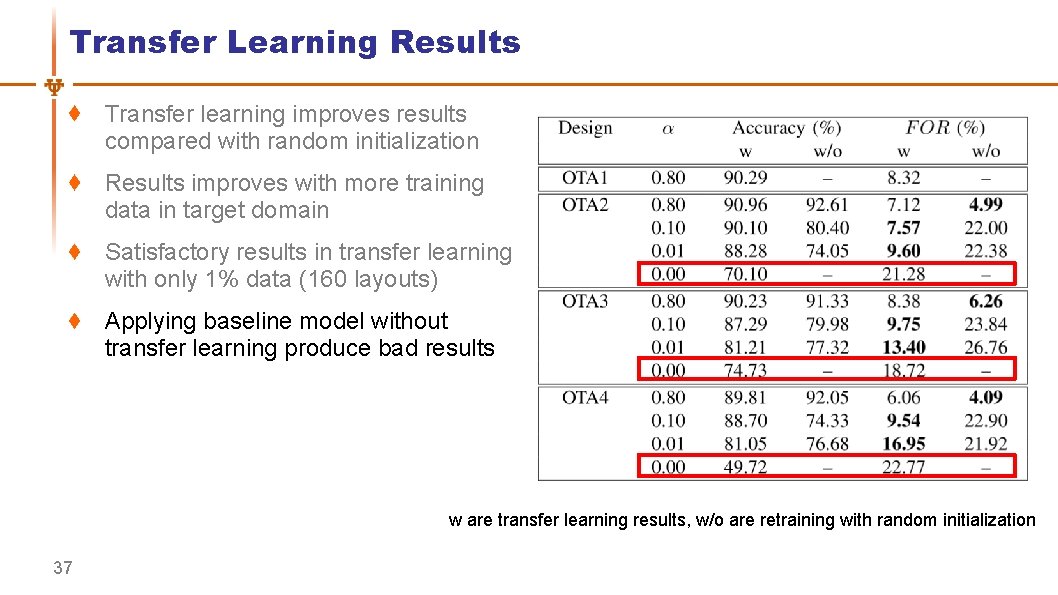
Transfer Learning Results Transfer learning improves results compared with random initialization Results improves with more training data in target domain Satisfactory results in transfer learning with only 1% data (160 layouts) w are transfer learning results, w/o are retraining with random initialization 36

Transfer Learning Results Transfer learning improves results compared with random initialization Results improves with more training data in target domain Satisfactory results in transfer learning with only 1% data (160 layouts) Applying baseline model without transfer learning produce bad results w are transfer learning results, w/o are retraining with random initialization 37

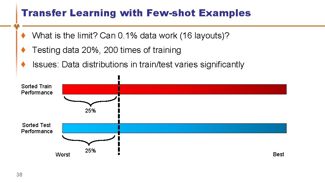
Transfer Learning with Few-shot Examples What is the limit? Can 0. 1% data work (16 layouts)? Testing data 20%, 200 times of training Issues: Data distributions in train/test varies significantly Sorted Train Performance 25% Sorted Test Performance Worst 38 25% Best

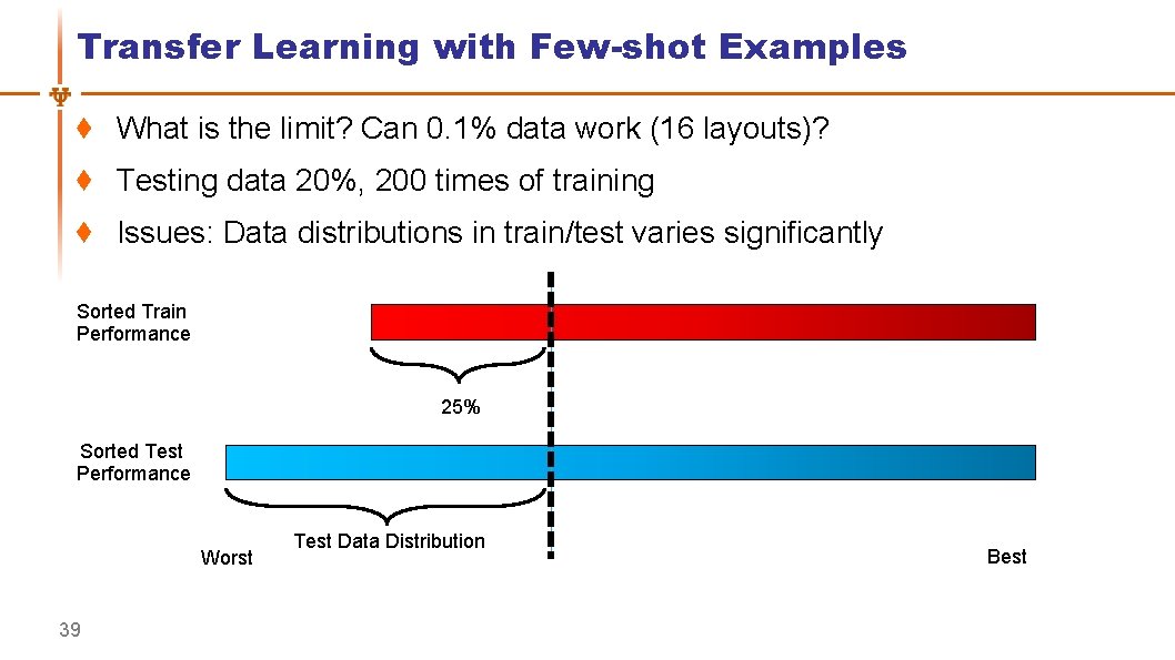
Transfer Learning with Few-shot Examples What is the limit? Can 0. 1% data work (16 layouts)? Testing data 20%, 200 times of training Issues: Data distributions in train/test varies significantly Sorted Train Performance 25% Sorted Test Performance Worst 39 Test Data Distribution Best

Transfer Learning with Few-shot Examples Random select 16 layouts (0. 1%) as transfer learning data Label training data according to relative rank in training set Relabel testing set according to the training set Repeat experiment for 100 times for each transfer target 40

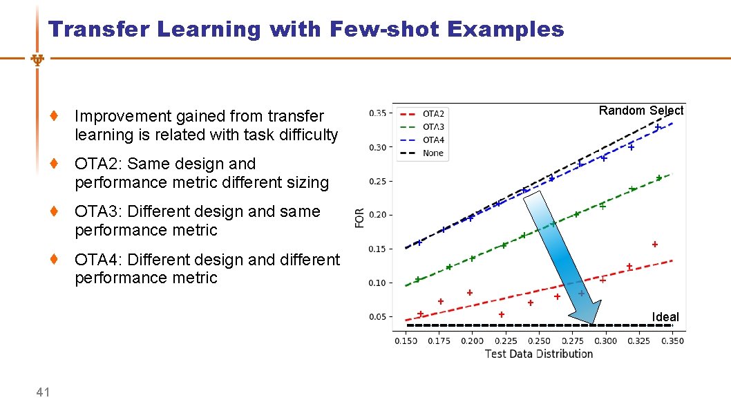
Transfer Learning with Few-shot Examples Improvement gained from transfer learning is related with task difficulty Random Select OTA 2: Same design and performance metric different sizing OTA 3: Different design and same performance metric OTA 4: Different design and different performance metric Ideal 41

Outline Introduction and Motivation UT-An. Lay Dataset with MAGICAL Placement Quality Prediction Improved Data Efficiency with Transfer Learning Conclusions 42

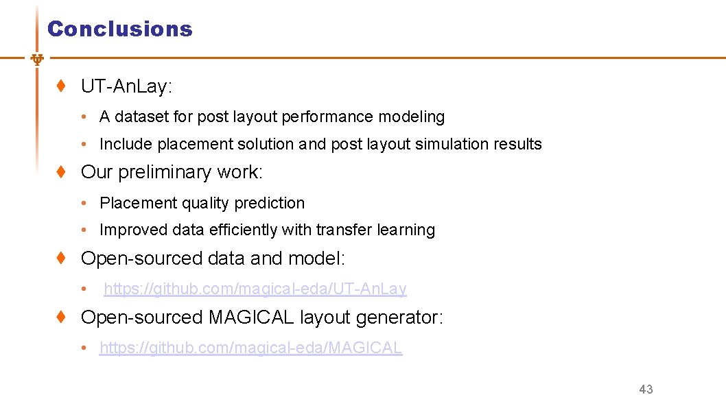
Conclusions UT-An. Lay: • A dataset for post layout performance modeling • Include placement solution and post layout simulation results Our preliminary work: • Placement quality prediction • Improved data efficiently with transfer learning Open-sourced data and model: • https: //github. com/magical-eda/UT-An. Lay Open-sourced MAGICAL layout generator: • https: //github. com/magical-eda/MAGICAL 43

Thank You 44