TOPIC5 SOFTWARE PROJECT PLANNING 1 Software Project Planning

TOPIC-5 SOFTWARE PROJECT PLANNING 1

Software Project Planning • The first step of software projects management process is the project planning step. • Project planning, in turn, start with Estimation. • Estimation is both an ‘art’ and ‘science’ (There are techniques for time and human-effort estimation) We have got to estimate: • resources, cost and schedule required for a Project. • Estimation requires experience access to info on previous projects. • Estimation carries a risk. • If we are familiar with the type of projects, we are going to handle, estimation becomes easier. 2

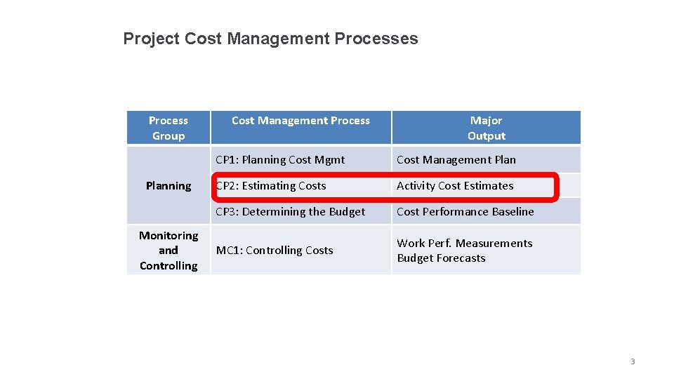
Project Cost Management Processes Process Group Planning Monitoring and Controlling Cost Management Process Major Output CP 1: Planning Cost Mgmt Cost Management Plan CP 2: Estimating Costs Activity Cost Estimates CP 3: Determining the Budget Cost Performance Baseline MC 1: Controlling Costs Work Perf. Measurements Budget Forecasts 3

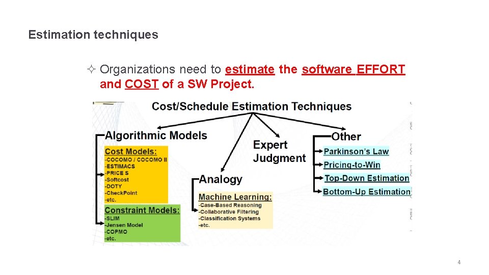
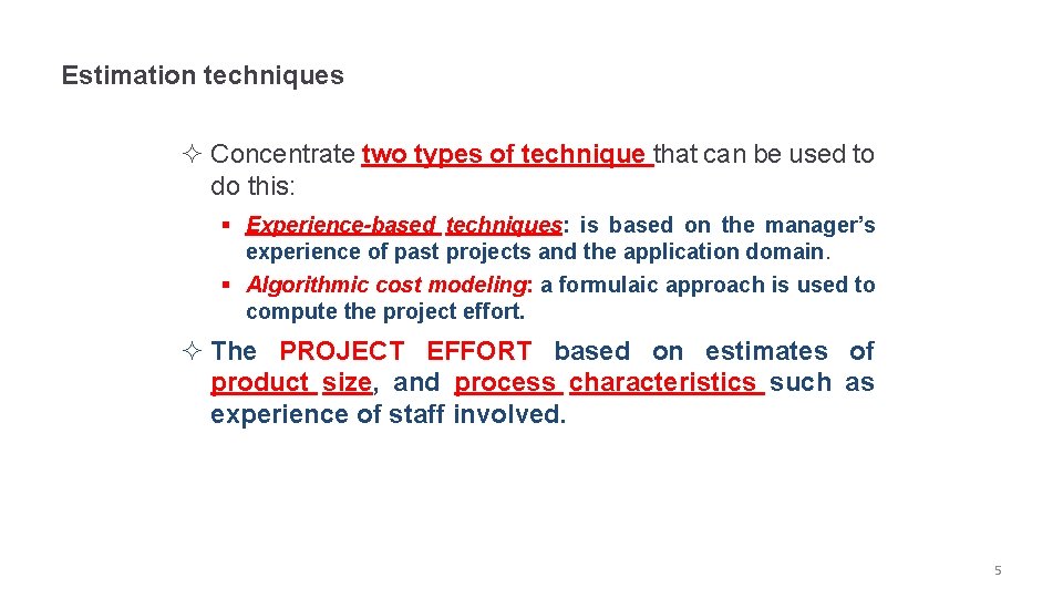
Estimation techniques ² Organizations need to estimate the software EFFORT and COST of a SW Project. 4

Estimation techniques ² Concentrate two types of technique that can be used to do this: § Experience-based techniques: is based on the manager’s experience of past projects and the application domain. § Algorithmic cost modeling: a formulaic approach is used to compute the project effort. ² The PROJECT EFFORT based on estimates of product size, and process characteristics such as experience of staff involved. 5

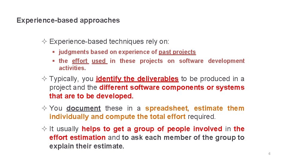
Experience-based approaches ² Experience-based techniques rely on: § judgments based on experience of past projects § the effort used in these projects on software development activities. ² Typically, you identify the deliverables to be produced in a project and the different software components or systems that are to be developed. ² You document these in a spreadsheet, estimate them individually and compute the total effort required. ² It usually helps to get a group of people involved in the effort estimation and to ask each member of the group to explain their estimate. 6

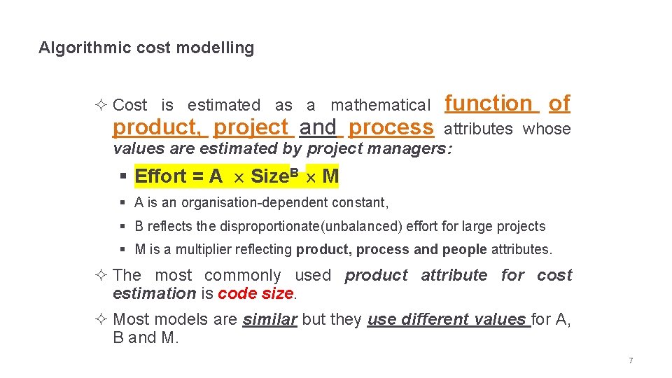
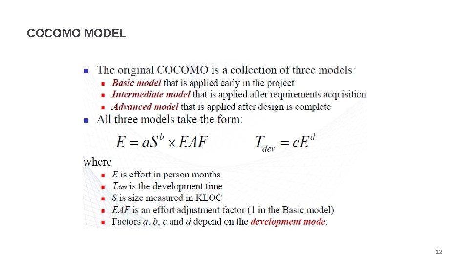
Algorithmic cost modelling ² Cost is estimated as a mathematical product, project and process function of attributes whose values are estimated by project managers: § Effort = A ´ Size. B ´ M § A is an organisation-dependent constant, § B reflects the disproportionate(unbalanced) effort for large projects § M is a multiplier reflecting product, process and people attributes. ² The most commonly used product attribute for cost estimation is code size. ² Most models are similar but they use different values for A, B and M. 7

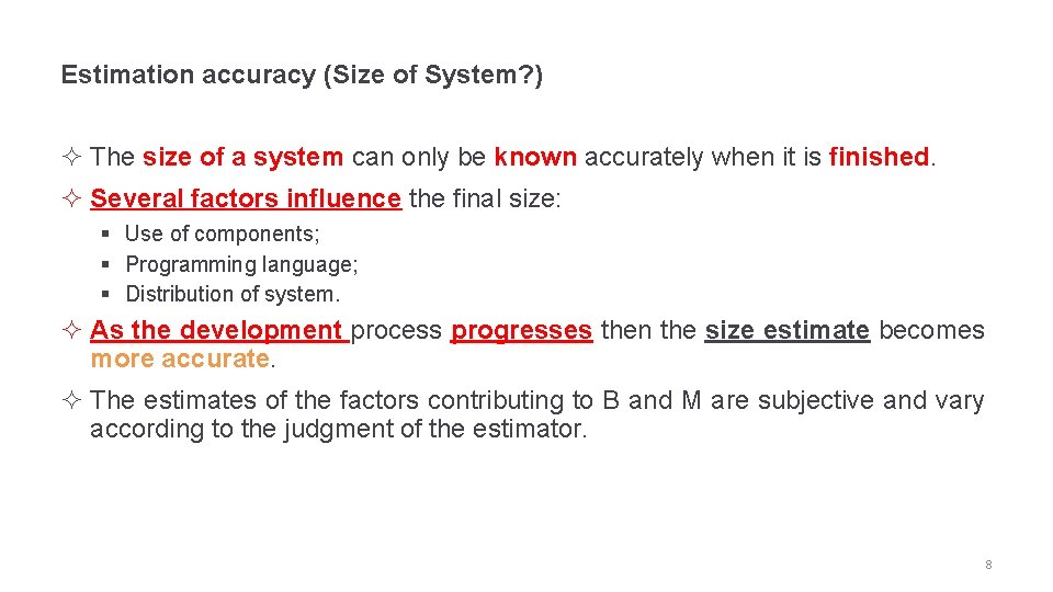
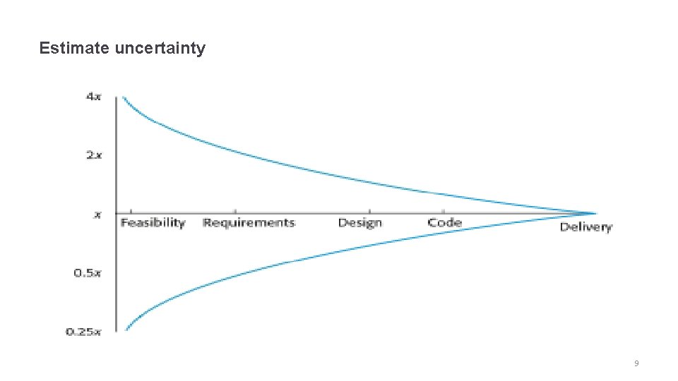
Estimation accuracy (Size of System? ) ² The size of a system can only be known accurately when it is finished. ² Several factors influence the final size: § Use of components; § Programming language; § Distribution of system. ² As the development process progresses then the size estimate becomes more accurate. ² The estimates of the factors contributing to B and M are subjective and vary according to the judgment of the estimator. 8

Estimate uncertainty 9

COCOMO Reading Overview of COCOMO ² http: //www. softstarsystems. com/overview. htm ² Copyright © 1986 -2015 Softstar Systems. All rights reserved. System. Star®, Costar™, and Calico™ are trademarks of Softstar Systems. 10

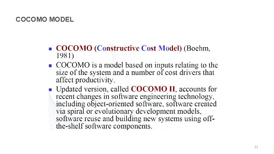
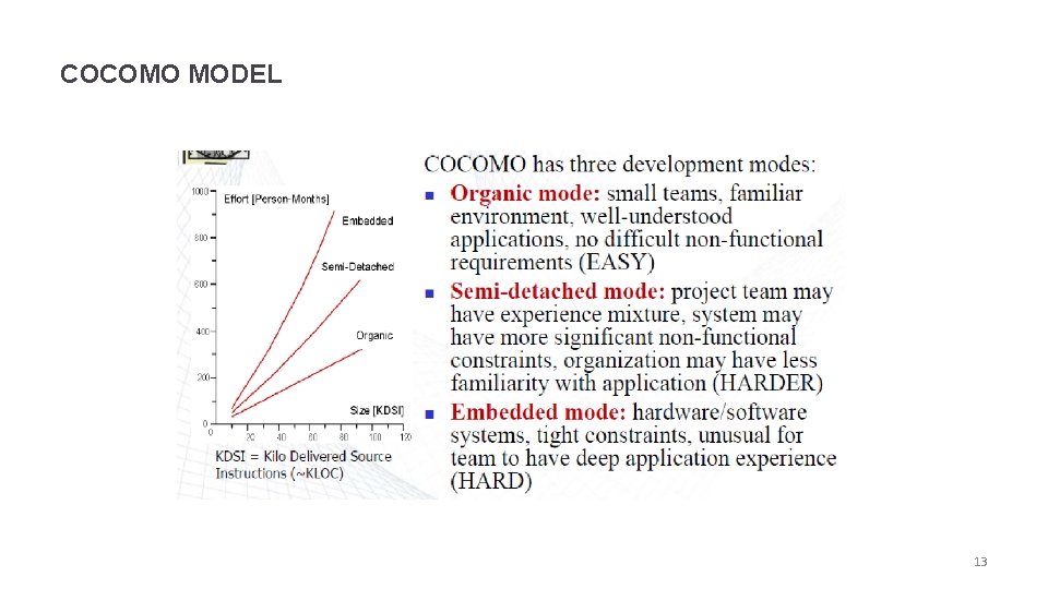
COCOMO MODEL 11

COCOMO MODEL 12

COCOMO MODEL 13

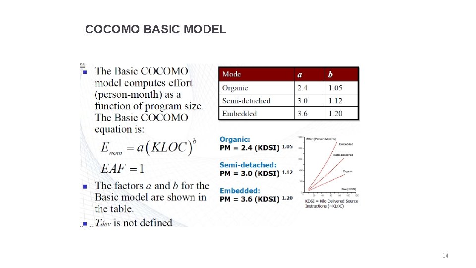
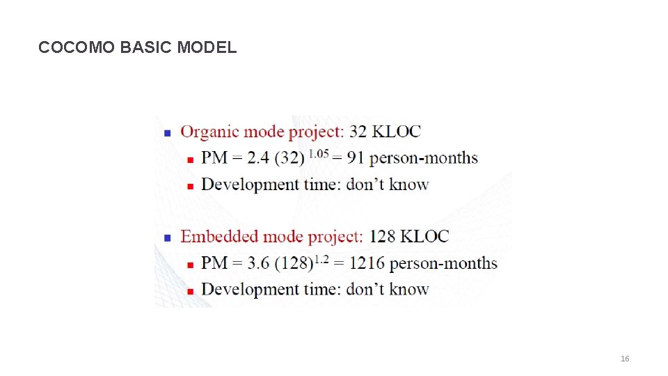
COCOMO BASIC MODEL 14

COCOMO BASIC MODEL 15

COCOMO BASIC MODEL 16

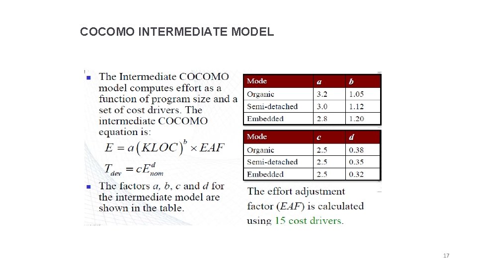
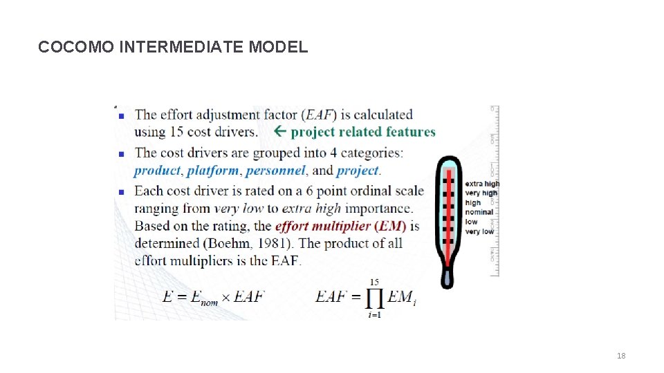
COCOMO INTERMEDIATE MODEL 17

COCOMO INTERMEDIATE MODEL 18

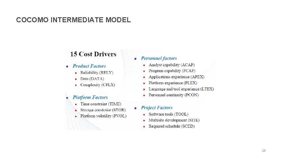
COCOMO INTERMEDIATE MODEL 19

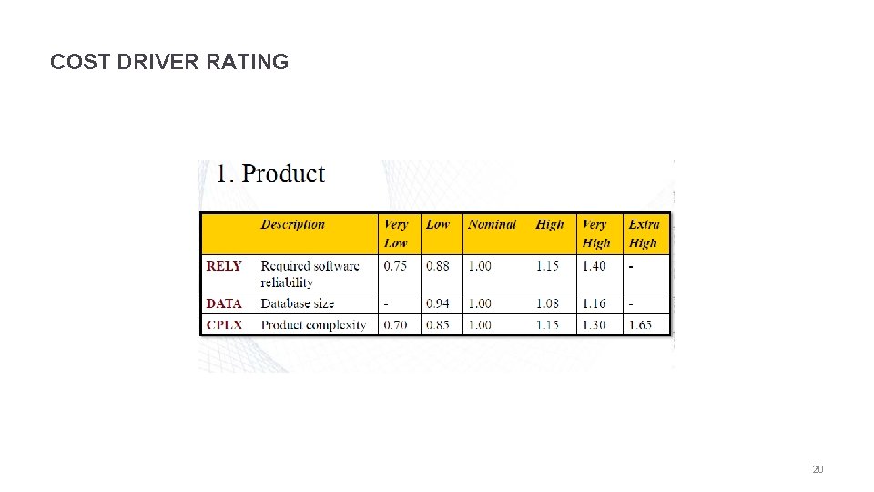
COST DRIVER RATING 20

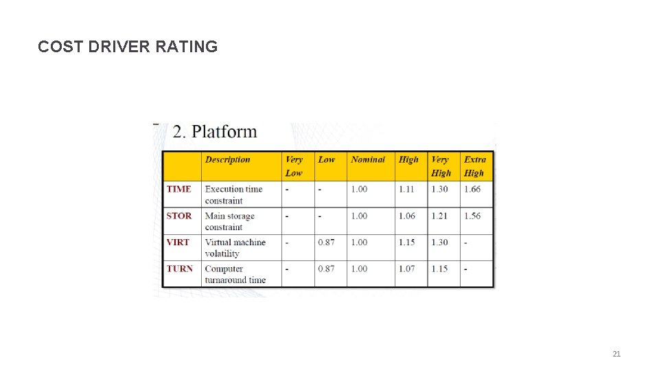
COST DRIVER RATING 21

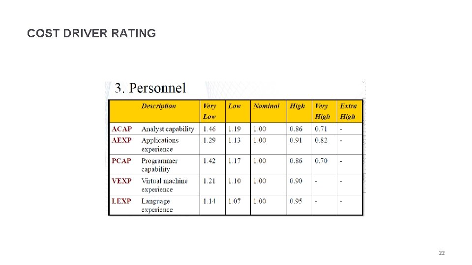
COST DRIVER RATING 22

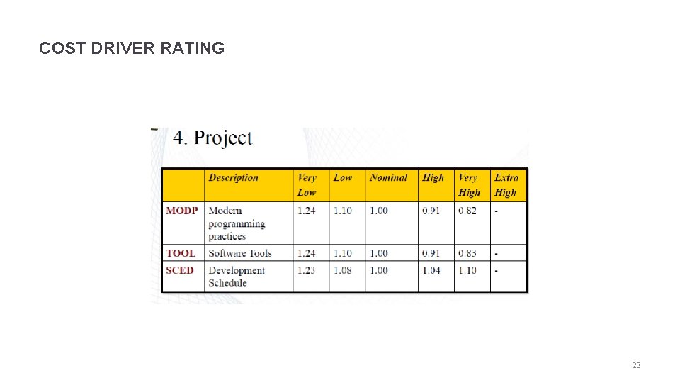
COST DRIVER RATING 23

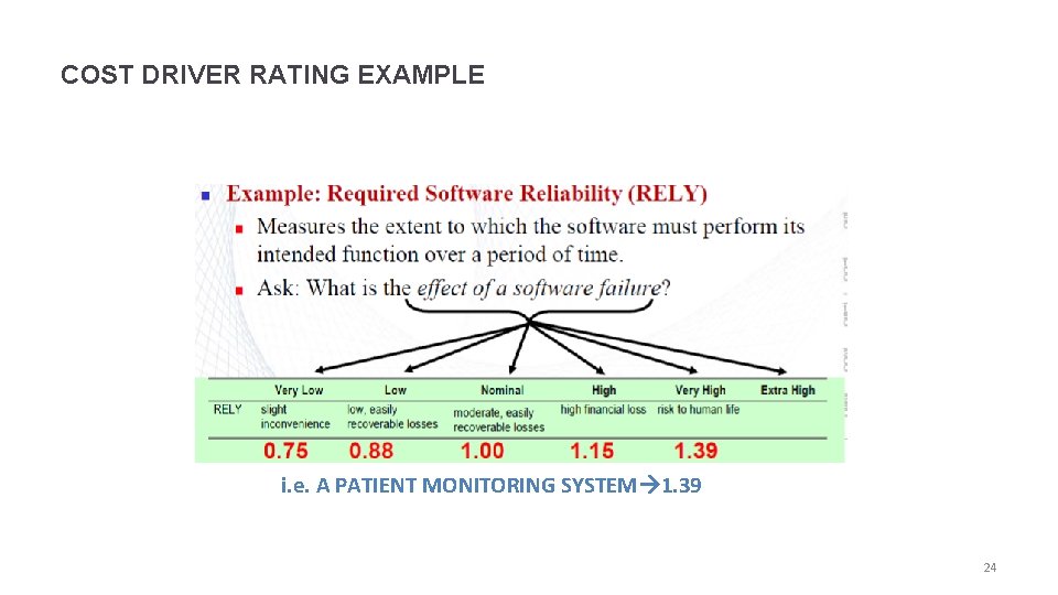
COST DRIVER RATING EXAMPLE i. e. A PATIENT MONITORING SYSTEM 1. 39 24

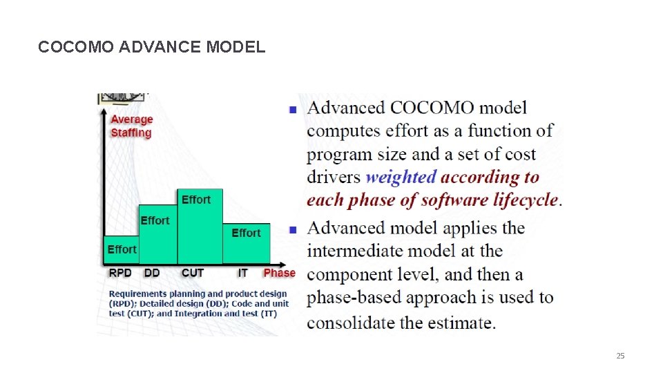
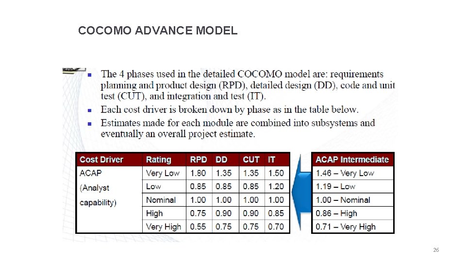
COCOMO ADVANCE MODEL 25

COCOMO ADVANCE MODEL 26

COCOMO II 27

COCOMO II 28

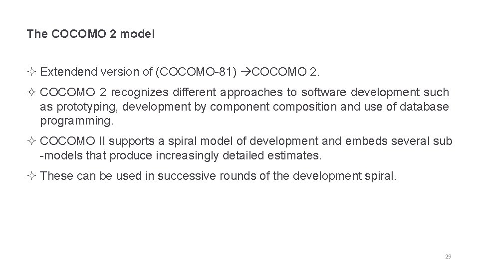
The COCOMO 2 model ² Extendend version of (COCOMO-81) COCOMO 2. ² COCOMO 2 recognizes different approaches to software development such as prototyping, development by component composition and use of database programming. ² COCOMO II supports a spiral model of development and embeds several sub -models that produce increasingly detailed estimates. ² These can be used in successive rounds of the development spiral. 29

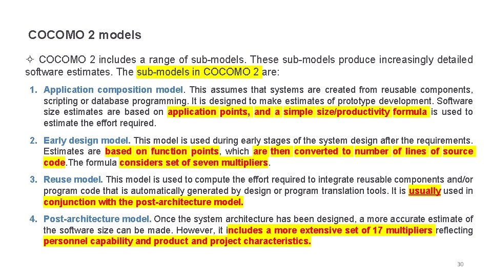
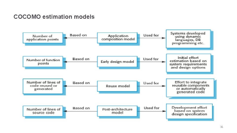
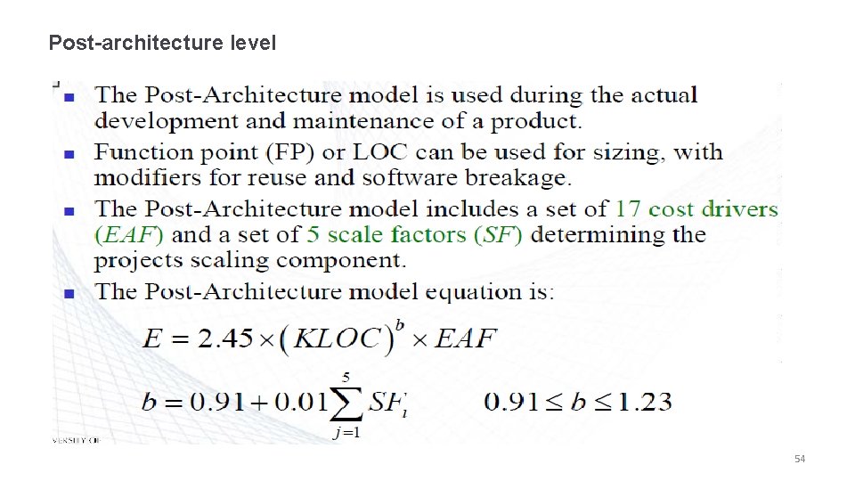
COCOMO 2 models ² COCOMO 2 includes a range of sub-models. These sub-models produce increasingly detailed software estimates. The sub-models in COCOMO 2 are: 1. Application composition model. This assumes that systems are created from reusable components, scripting or database programming. It is designed to make estimates of prototype development. Software size estimates are based on application points, and a simple size/productivity formula is used to estimate the effort required. 2. Early design model. This model is used during early stages of the system design after the requirements. Estimates are based on function points, which are then converted to number of lines of source code. The formula considers set of seven multipliers. 3. Reuse model. This model is used to compute the effort required to integrate reusable components and/or program code that is automatically generated by design or program translation tools. It is usually used in conjunction with the post-architecture model. 4. Post-architecture model. Once the system architecture has been designed, a more accurate estimate of the software size can be made. However, it includes a more extensive set of 17 multipliers reflecting personnel capability and product and project characteristics. 30

COCOMO estimation models 31

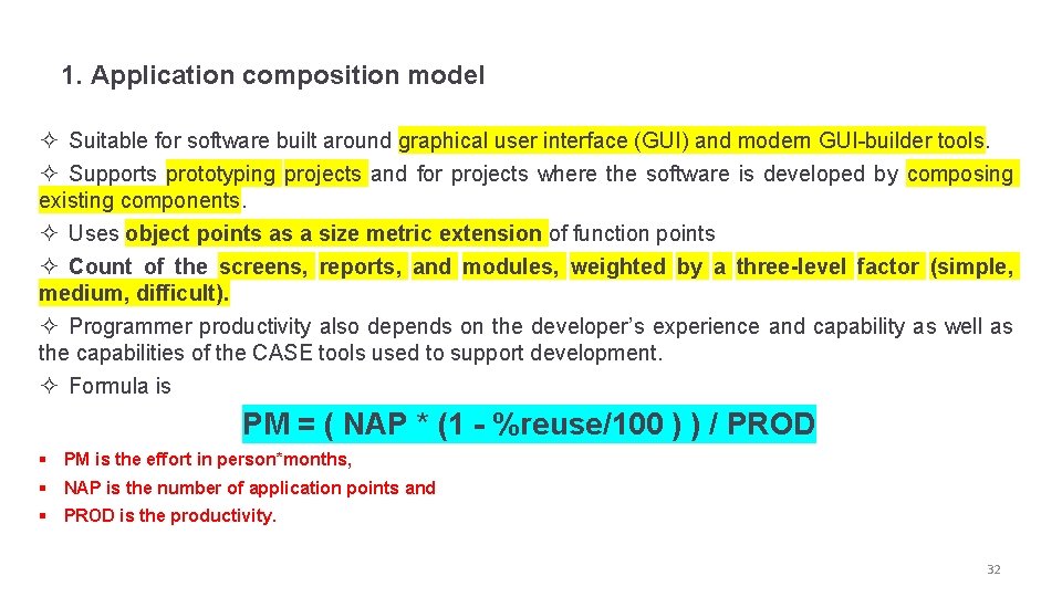
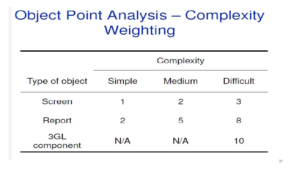
1. Application composition model ² Suitable for software built around graphical user interface (GUI) and modern GUI-builder tools. ² Supports prototyping projects and for projects where the software is developed by composing existing components. ² Uses object points as a size metric extension of function points ² Count of the screens, reports, and modules, weighted by a three-level factor (simple, medium, difficult). ² Programmer productivity also depends on the developer’s experience and capability as well as the capabilities of the CASE tools used to support development. ² Formula is PM = ( NAP * (1 - %reuse/100 ) ) / PROD § PM is the effort in person*months, § NAP is the number of application points and § PROD is the productivity. 32

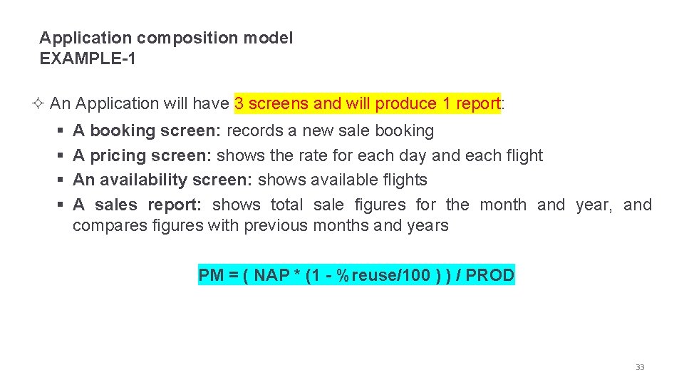
Application composition model EXAMPLE-1 ² An Application will have 3 screens and will produce 1 report: § § A booking screen: records a new sale booking A pricing screen: shows the rate for each day and each flight An availability screen: shows available flights A sales report: shows total sale figures for the month and year, and compares figures with previous months and years PM = ( NAP * (1 - %reuse/100 ) ) / PROD 33

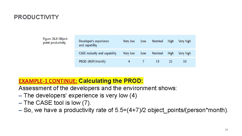
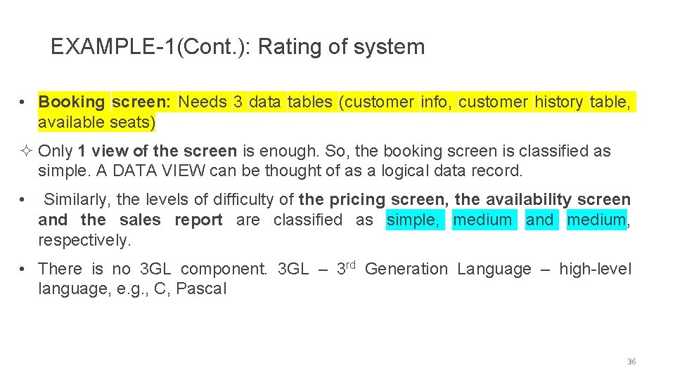
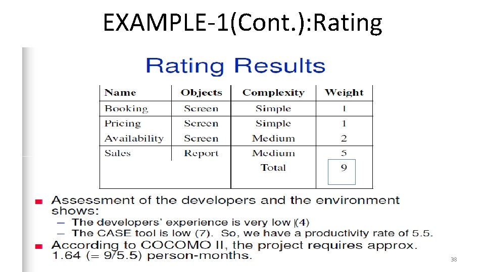
PRODUCTIVITY EXAMPLE-1 CONTINUE: Calculating the PROD: Assessment of the developers and the environment shows: – The developers’ experience is very low (4) – The CASE tool is low (7). – So, we have a productivity rate of 5. 5=(4+7)/2 object_points/(person*month). 34

35

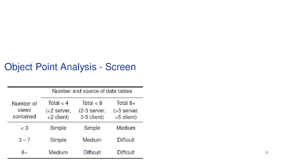
EXAMPLE-1(Cont. ): Rating of system • Booking screen: Needs 3 data tables (customer info, customer history table, available seats) ² Only 1 view of the screen is enough. So, the booking screen is classified as simple. A DATA VIEW can be thought of as a logical data record. • Similarly, the levels of difficulty of the pricing screen, the availability screen and the sales report are classified as simple, medium and medium, respectively. • There is no 3 GL component. 3 GL – 3 rd Generation Language – high-level language, e. g. , C, Pascal 36

37

EXAMPLE-1(Cont. ): Rating 38

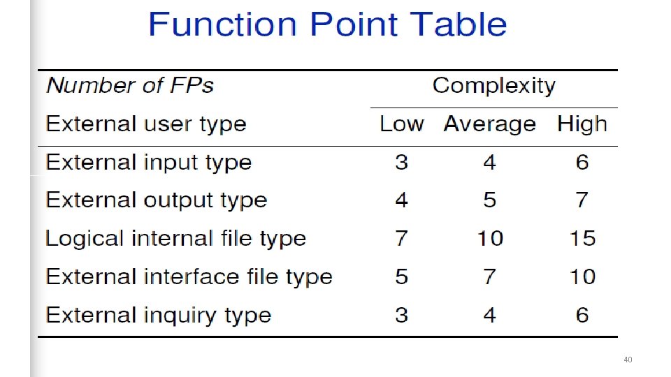
CONVERT OBJECT POINTS TO FUNCTIONAL POINTS 39

40

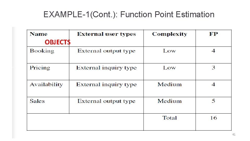
EXAMPLE-1(Cont. ): Function Point Estimation OBJECTS 41

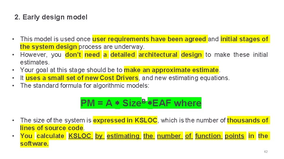
2. Early design model • This model is used once user requirements have been agreed and initial stages of the system design process are underway. • However, you don’t need a detailed architectural design to make these initial estimates. • Your goal at this stage should be to make an approximate estimate. • It uses a small set of new Cost Drivers, and new estimating equations. • The standard formula for algorithmic models: PM = A * Size. B *EAF where • The size of the system is expressed in KSLOC, which is the number of thousands of lines of source code. • You calculate KSLOC by estimating the number of function points in the software. 42

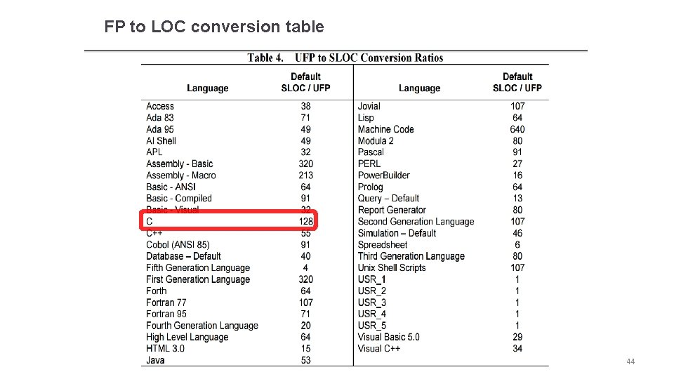
CONVERT FUNCTIONAL POINTS TO LOC 43

FP to LOC conversion table a 44

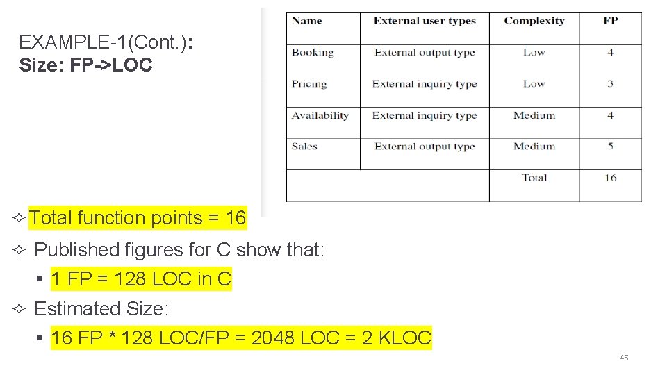
EXAMPLE-1(Cont. ): Size: FP->LOC ² Total function points = 16 ² Published figures for C show that: § 1 FP = 128 LOC in C ² Estimated Size: § 16 FP * 128 LOC/FP = 2048 LOC = 2 KLOC 45

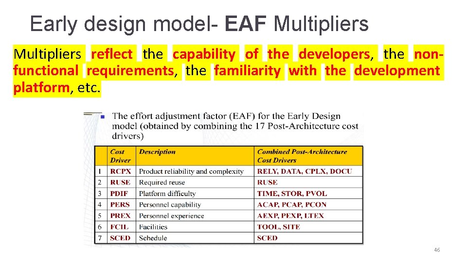
Early design model- EAF Multipliers reflect the capability of the developers, the nonfunctional requirements, the familiarity with the development platform, etc. 46

47

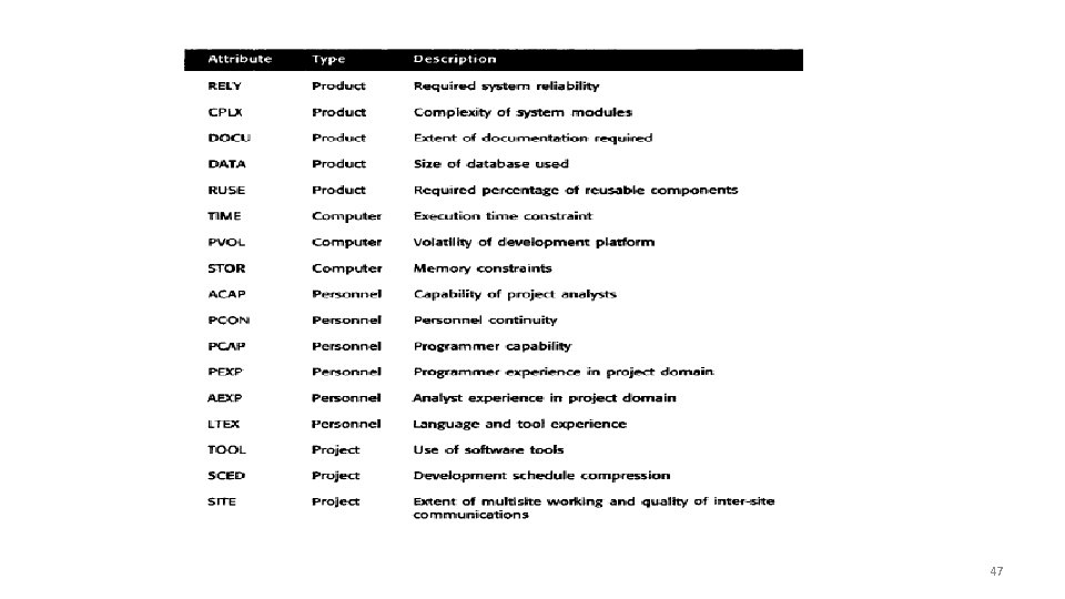
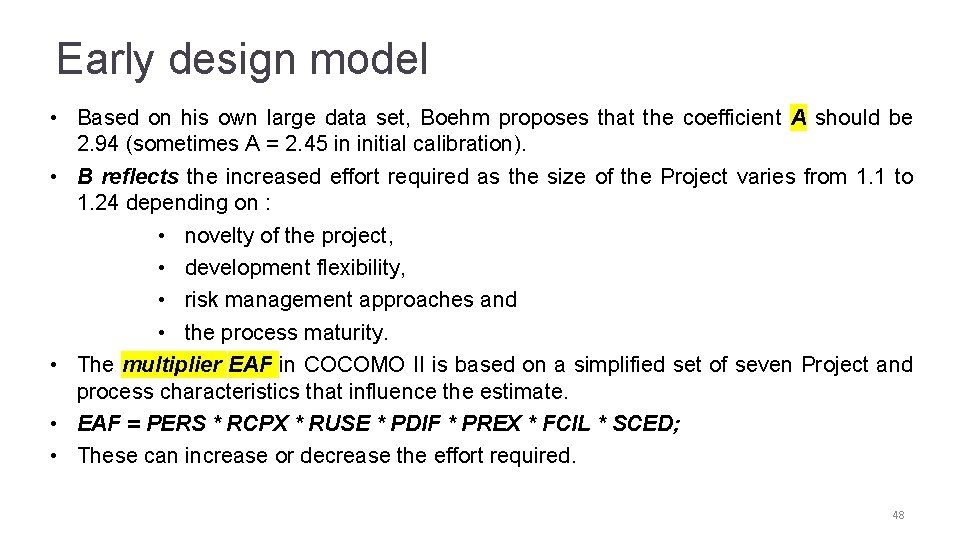
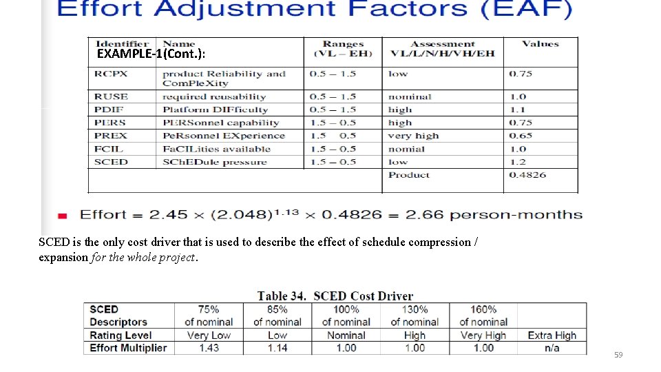
Early design model • Based on his own large data set, Boehm proposes that the coefficient A should be 2. 94 (sometimes A = 2. 45 in initial calibration). • B reflects the increased effort required as the size of the Project varies from 1. 1 to 1. 24 depending on : • novelty of the project, • development flexibility, • risk management approaches and • the process maturity. • The multiplier EAF in COCOMO II is based on a simplified set of seven Project and process characteristics that influence the estimate. • EAF = PERS * RCPX * RUSE * PDIF * PREX * FCIL * SCED; • These can increase or decrease the effort required. 48

3. The reuse model • Software reuse is now common, and most large systems include a significant percentage of code that is reused from previous developments. • The reuse model is used to estimate the effort required to integrate reusable or generated code. 49

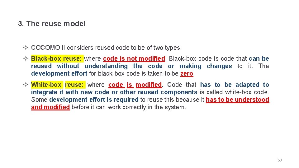
3. The reuse model ² COCOMO II considers reused code to be of two types. ² Black-box reuse: where code is not modified. Black-box code is code that can be reused without understanding the code or making changes to it. The development effort for black-box code is taken to be zero. ² White-box reuse: where code is modified. Code that has to be adapted to integrate it with new code or other reused components is called white-box code. Some development effort is required to reuse this because it has to be understood and modified before it can work correctly in the system. 50

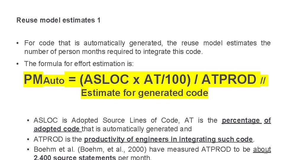
Reuse model estimates 1 • For code that is automatically generated, the reuse model estimates the number of person months required to integrate this code. • The formula for effort estimation is: PMAuto = (ASLOC x AT/100) / ATPROD // Estimate for generated code • ASLOC is Adopted Source Lines of Code, AT is the percentage of adopted code that is automatically generated and • ATPROD is the productivity of engineers in integrating such code. • Boehm et al. (Boehm, et al. , 2000) have measured ATPROD to be about 51

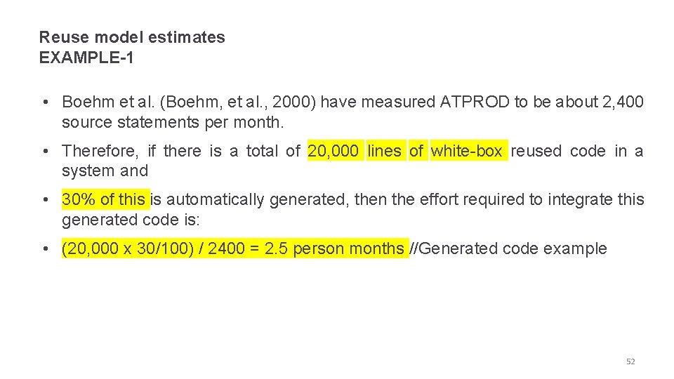
Reuse model estimates EXAMPLE-1 • Boehm et al. (Boehm, et al. , 2000) have measured ATPROD to be about 2, 400 source statements per month. • Therefore, if there is a total of 20, 000 lines of white-box reused code in a system and • 30% of this is automatically generated, then the effort required to integrate this generated code is: • (20, 000 x 30/100) / 2400 = 2. 5 person months //Generated code example 52

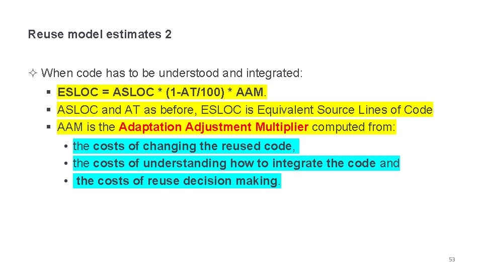
Reuse model estimates 2 ² When code has to be understood and integrated: § ESLOC = ASLOC * (1 -AT/100) * AAM. § ASLOC and AT as before, ESLOC is Equivalent Source Lines of Code § AAM is the Adaptation Adjustment Multiplier computed from: • the costs of changing the reused code, • the costs of understanding how to integrate the code and • the costs of reuse decision making. 53

Post-architecture level 54

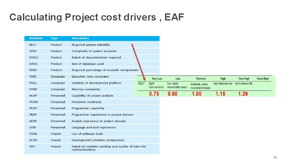
Calculating Project cost drivers , EAF 55

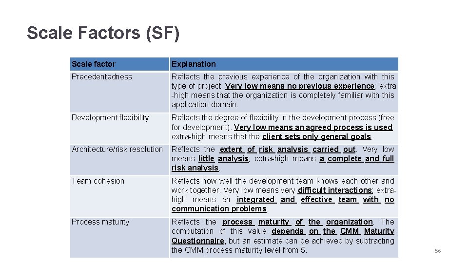
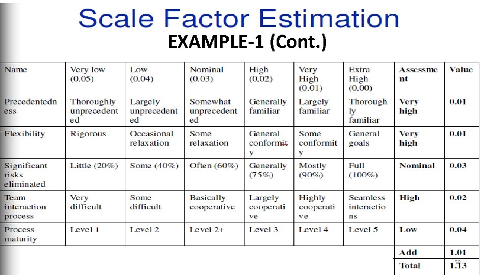
Scale Factors (SF) Scale factor Explanation Precedentedness Reflects the previous experience of the organization with this type of project. Very low means no previous experience; extra -high means that the organization is completely familiar with this application domain. Development flexibility Reflects the degree of flexibility in the development process (free for development). Very low means an agreed process is used; extra-high means that the client sets only general goals. Architecture/risk resolution Reflects the extent of risk analysis carried out. Very low means little analysis; extra-high means a complete and full risk analysis. Team cohesion Reflects how well the development team knows each other and work together. Very low means very difficult interactions; extrahigh means an integrated and effective team with no communication problems. Process maturity Reflects the process maturity of the organization. The computation of this value depends on the CMM Maturity Questionnaire, but an estimate can be achieved by subtracting the CMM process maturity level from 5. 56

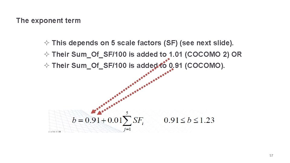
The exponent term ² This depends on 5 scale factors (SF) (see next slide). ² Their Sum_Of_SF/100 is added to 1. 01 (COCOMO 2) OR ² Their Sum_Of_SF/100 is added to 0. 91 (COCOMO). 57

EXAMPLE-1 (Cont. ) 58

EXAMPLE-1(Cont. ): SCED is the only cost driver that is used to describe the effect of schedule compression / expansion for the whole project. 59

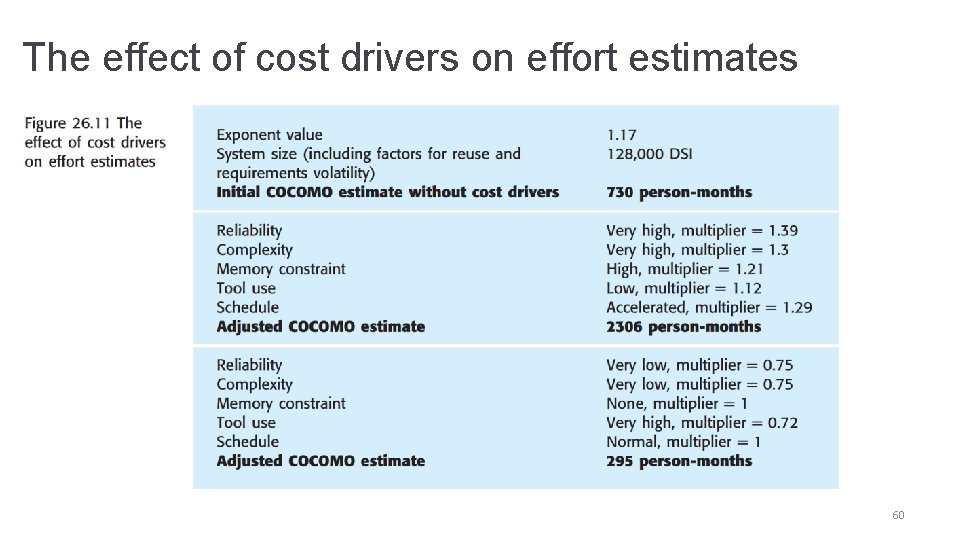
The effect of cost drivers on effort estimates 60

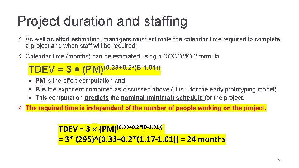
Project duration and staffing ² As well as effort estimation, managers must estimate the calendar time required to complete a project and when staff will be required. ² Calendar time (months) can be estimated using a COCOMO 2 formula TDEV = 3 * (PM)(0. 33+0. 2*(B-1. 01)) § PM is the effort computation and § B is the exponent computed as discussed above (B is 1 for the early prototyping model). § This computation predicts the nominal (minimal) schedule for the project. ² The required time is independent of the number of people working on the project. TDEV = 3 ´ (PM)(0. 33+0. 2*(B-1. 01)) = 3* (295)^(0. 33+0. 2*(1. 17 -1. 01)) = 24 months 61

Staffing requirements ² required staff can’t be computed by dividing the development time by the required schedule. ² The number of people working on a project varies depending on the phase of the project. ² The more people who work on the project, the more total effort is usually required. ² A very rapid build-up of people often correlates with schedule slippage. 62

Key points ² Estimation techniques for software may be experience-based, where managers judge the effort required, or algorithmic, where the effort required is computed from other estimated project parameters. ² The COCOMO II costing model is an algorithmic cost model that uses project, product, hardware and personnel attributes as well as product size and complexity attributes to derive a cost estimate. 63

Cocomo II-Tool Usage. Example Screens Homework: Use it for your Project Estimation! 64

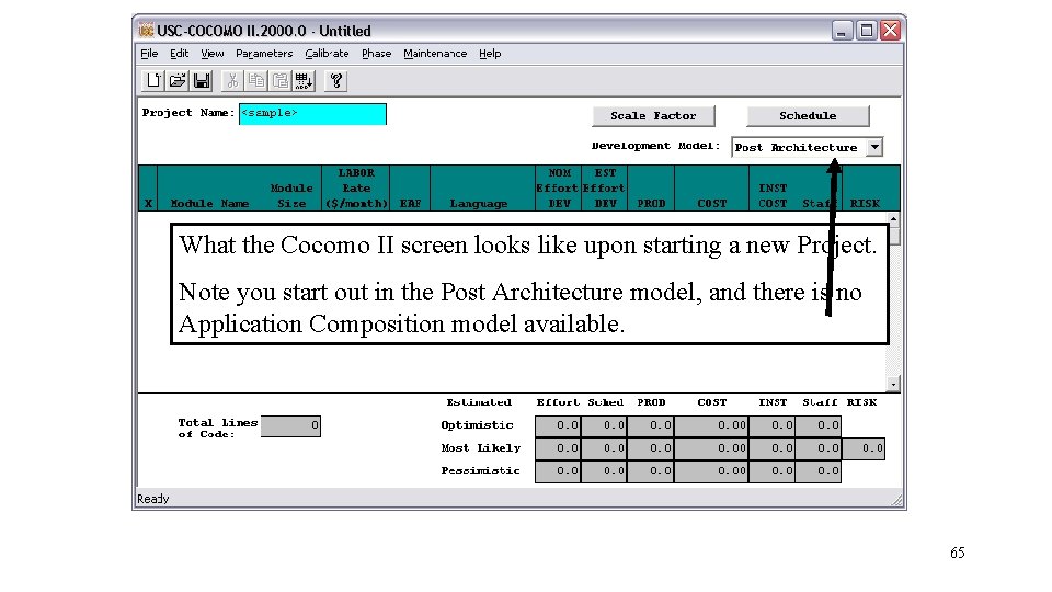
What the Cocomo II screen looks like upon starting a new Project. Note you start out in the Post Architecture model, and there is no Application Composition model available. 65

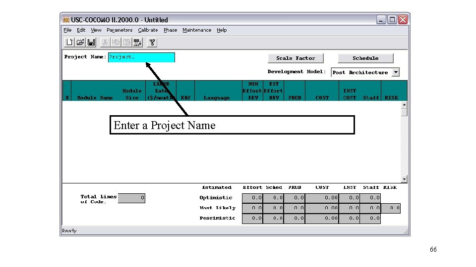
Enter a Project Name 66

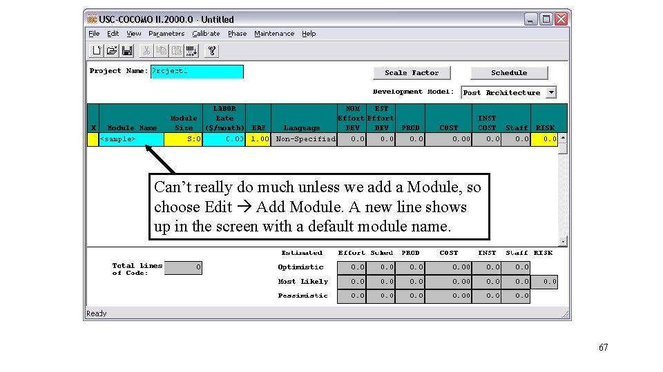
Can’t really do much unless we add a Module, so choose Edit Add Module. A new line shows up in the screen with a default module name. 67

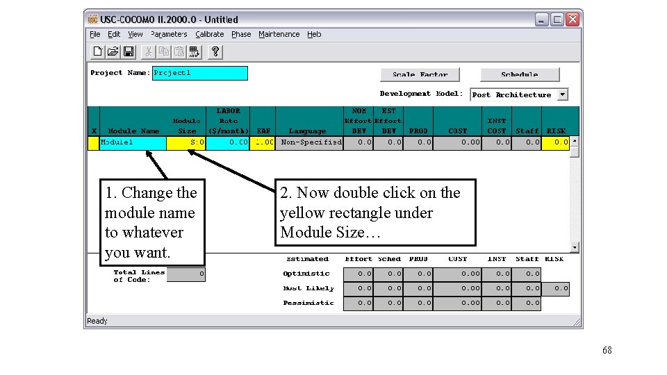
1. Change the module name to whatever you want. 2. Now double click on the yellow rectangle under Module Size… 68

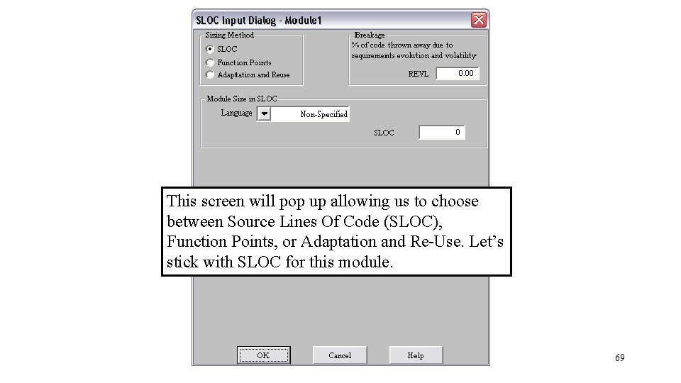
This screen will pop up allowing us to choose between Source Lines Of Code (SLOC), Function Points, or Adaptation and Re-Use. Let’s stick with SLOC for this module. 69

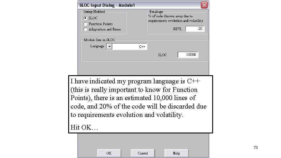
I have indicated my program language is C++ (this is really important to know for Function Points), there is an estimated 10, 000 lines of code, and 20% of the code will be discarded due to requirements evolution and volatility. Hit OK… 70

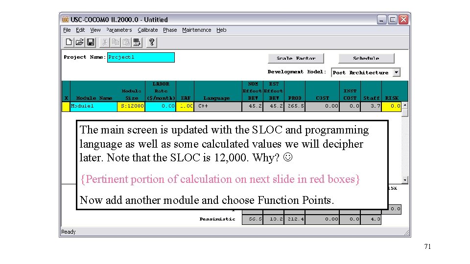
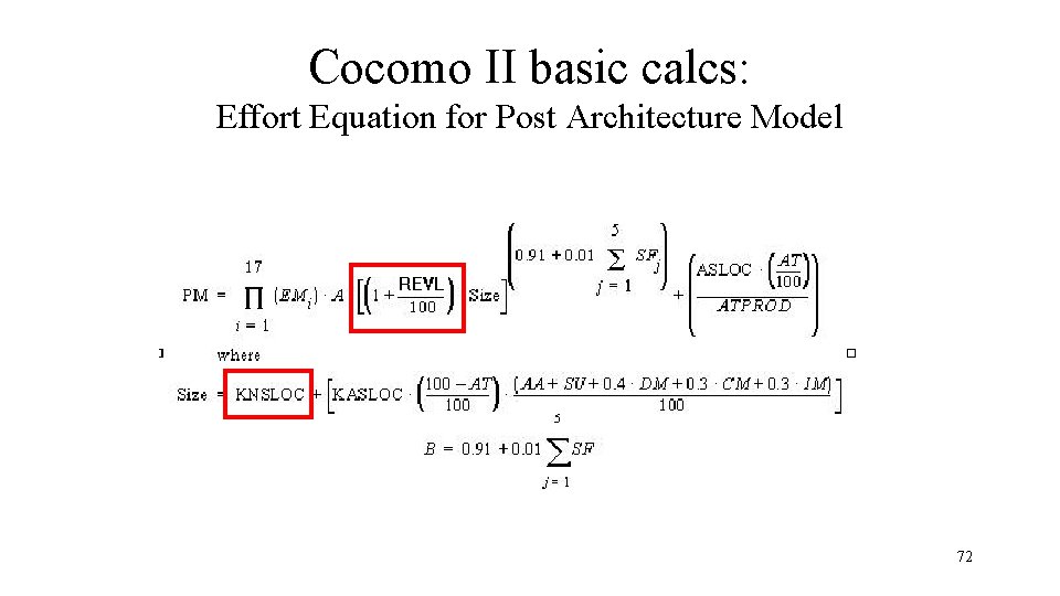
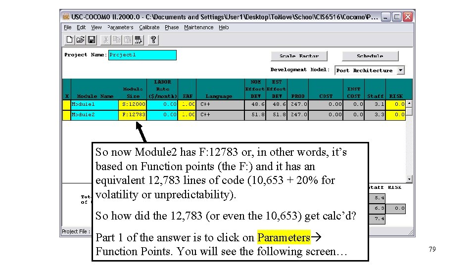
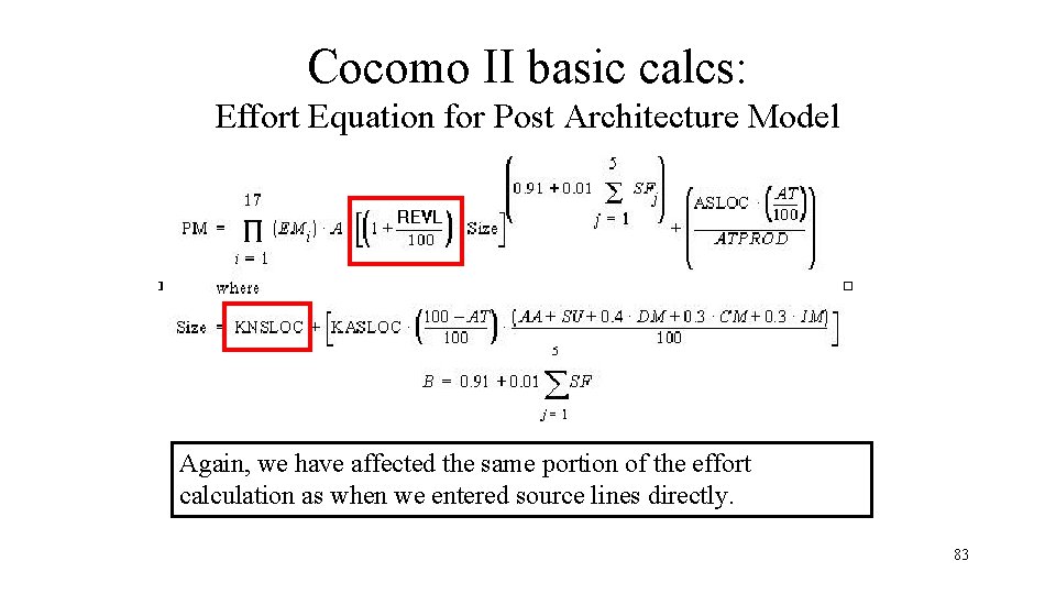
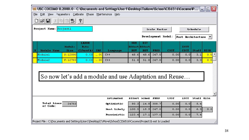
The main screen is updated with the SLOC and programming language as well as some calculated values we will decipher later. Note that the SLOC is 12, 000. Why? {Pertinent portion of calculation on next slide in red boxes} Now add another module and choose Function Points. 71

Cocomo II basic calcs: Effort Equation for Post Architecture Model 72

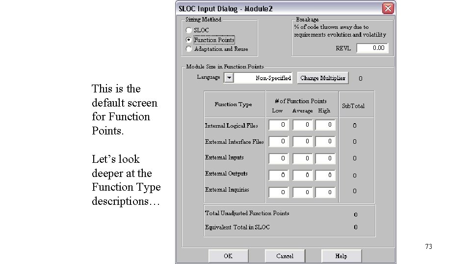
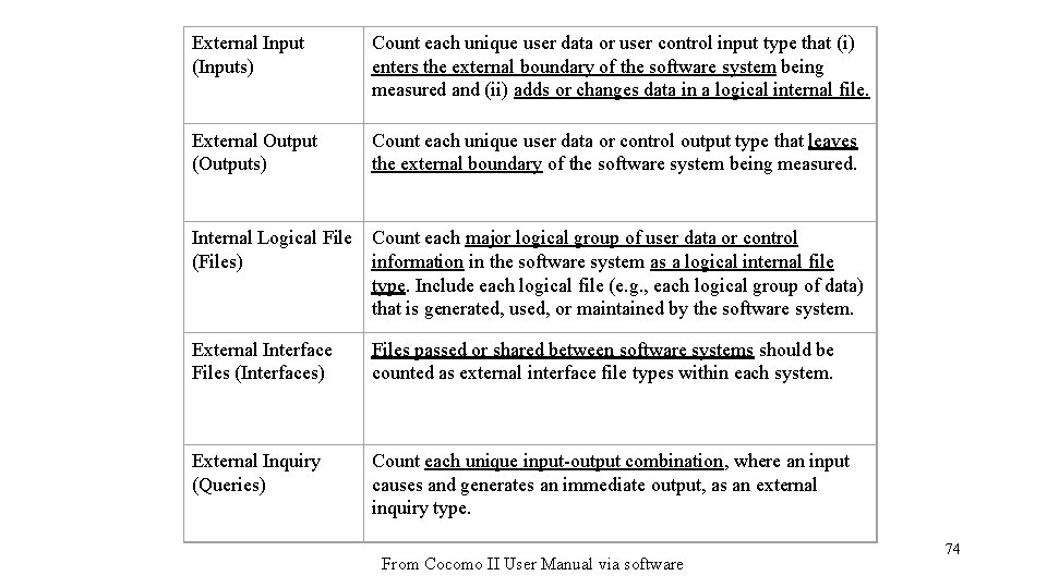
This is the default screen for Function Points. Let’s look deeper at the Function Type descriptions… 73

External Input (Inputs) Count each unique user data or user control input type that (i) enters the external boundary of the software system being measured and (ii) adds or changes data in a logical internal file. External Output (Outputs) Count each unique user data or control output type that leaves the external boundary of the software system being measured. Internal Logical File Count each major logical group of user data or control (Files) information in the software system as a logical internal file type. Include each logical file (e. g. , each logical group of data) that is generated, used, or maintained by the software system. External Interface Files (Interfaces) Files passed or shared between software systems should be counted as external interface file types within each system. External Inquiry (Queries) Count each unique input-output combination, where an input causes and generates an immediate output, as an external inquiry type. From Cocomo II User Manual via software 74

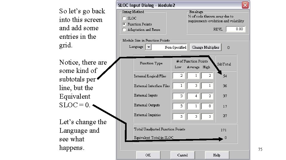
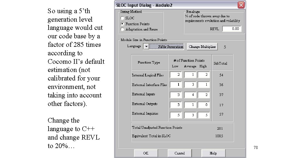
So let’s go back into this screen and add some entries in the grid. Notice, there are some kind of subtotals per line, but the Equivalent SLOC = 0. Let’s change the Language and see what happens. 75

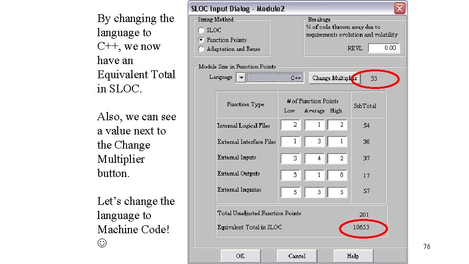
By changing the language to C++, we now have an Equivalent Total in SLOC. Also, we can see a value next to the Change Multiplier button. Let’s change the language to Machine Code! 76

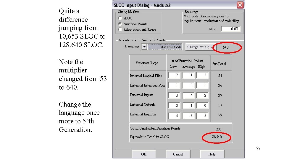
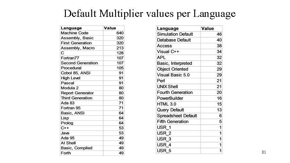
Quite a difference jumping from 10, 653 SLOC to 128, 640 SLOC. Note the multiplier changed from 53 to 640. Change the language once more to 5’th Generation. 77

So using a 5’th generation level language would cut our code base by a factor of 285 times according to Cocomo II’s default estimation (not calibrated for your environment, not taking into account other factors). Change the language to C++ and change REVL to 20%… 78

So now Module 2 has F: 12783 or, in other words, it’s based on Function points (the F: ) and it has an equivalent 12, 783 lines of code (10, 653 + 20% for volatility or unpredictability). So how did the 12, 783 (or even the 10, 653) get calc’d? Part 1 of the answer is to click on Parameters Function Points. You will see the following screen… 79

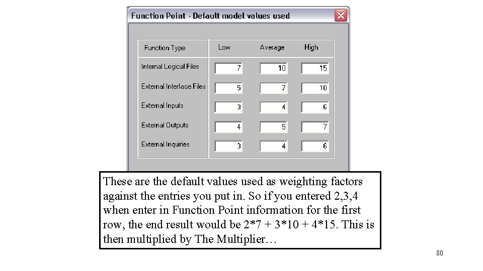
These are the default values used as weighting factors against the entries you put in. So if you entered 2, 3, 4 when enter in Function Point information for the first row, the end result would be 2*7 + 3*10 + 4*15. This is then multiplied by The Multiplier… 80

Default Multiplier values per Language 81

So let’s see what part of the calculation we just affected… 82

Cocomo II basic calcs: Effort Equation for Post Architecture Model Again, we have affected the same portion of the effort calculation as when we entered source lines directly. 83

So now let’s add a module and use Adaptation and Reuse… 84

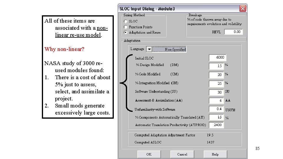
All of these items are associated with a nonlinear re-use model. Why non-linear? NASA study of 3000 reused modules found: 1. There is a cost of about 5% just to assess, select, and assimilate a project. 2. Small mods generate excessively large costs. 85

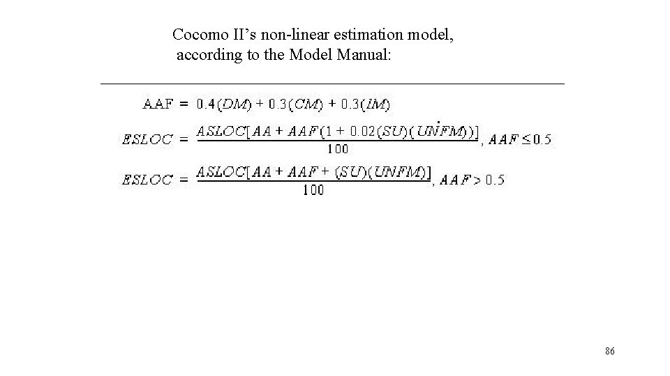
Cocomo II’s non-linear estimation model, according to the Model Manual: 86

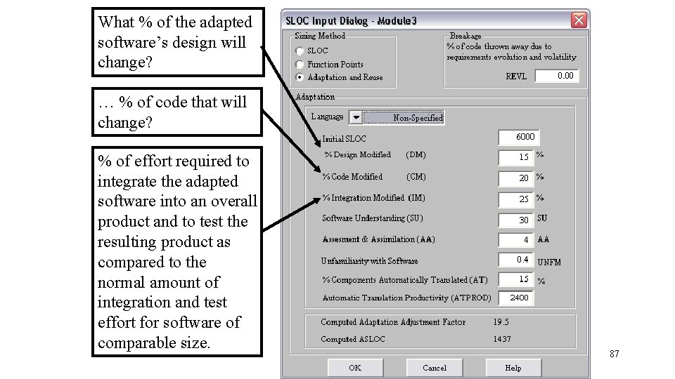
What % of the adapted software’s design will change? … % of code that will change? % of effort required to integrate the adapted software into an overall product and to test the resulting product as compared to the normal amount of integration and test effort for software of comparable size. 87

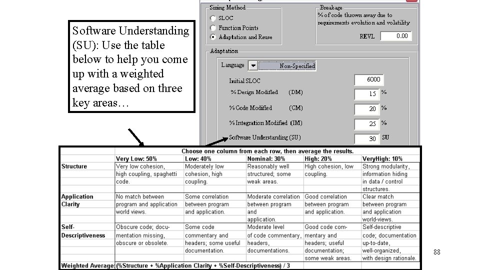
Software Understanding (SU): Use the table below to help you come up with a weighted average based on three key areas… 88

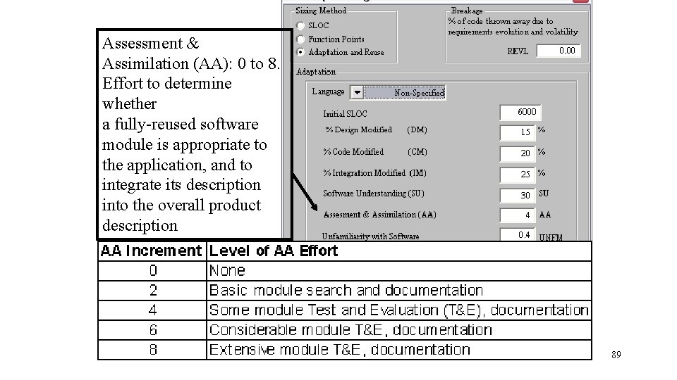
Assessment & Assimilation (AA): 0 to 8. Effort to determine whether a fully-reused software module is appropriate to the application, and to integrate its description into the overall product description 89

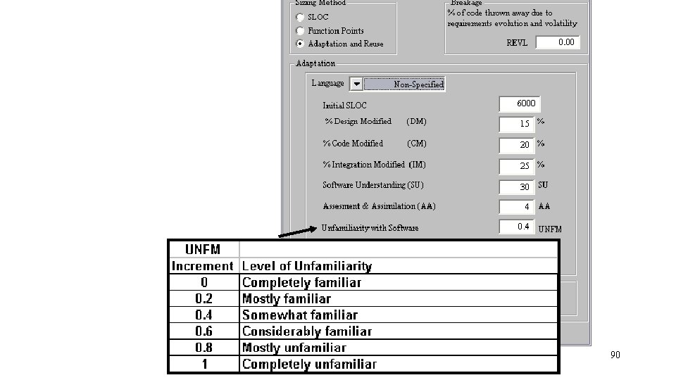
90

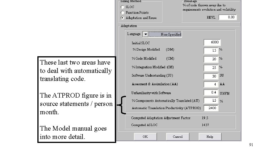
These last two areas have to deal with automatically translating code. The ATPROD figure is in source statements / person month. The Model manual goes into more detail. 91

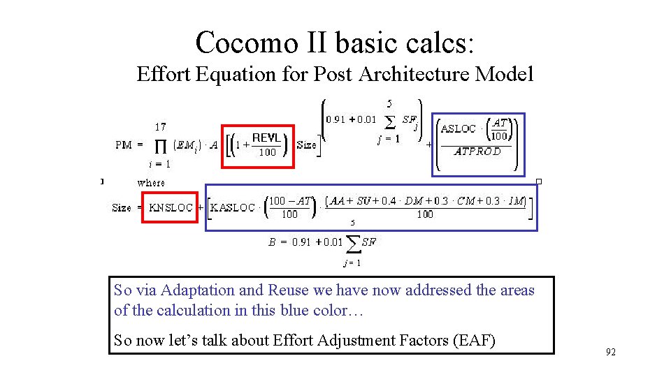
Cocomo II basic calcs: Effort Equation for Post Architecture Model So via Adaptation and Reuse we have now addressed the areas of the calculation in this blue color… So now let’s talk about Effort Adjustment Factors (EAF) 92

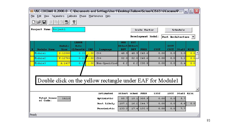
Double click on the yellow rectangle under EAF for Module 1 93

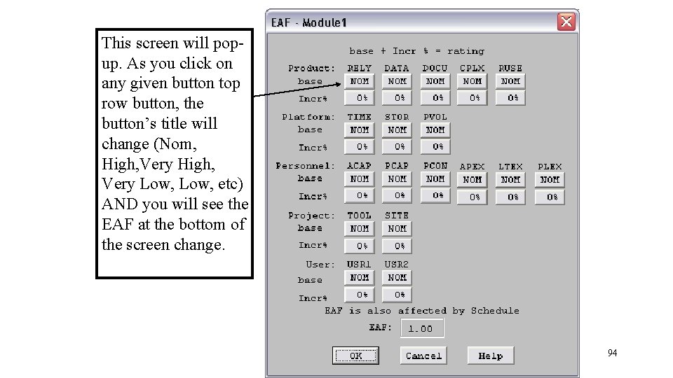
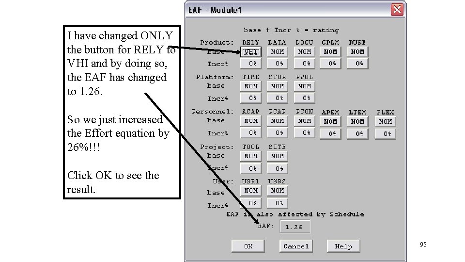
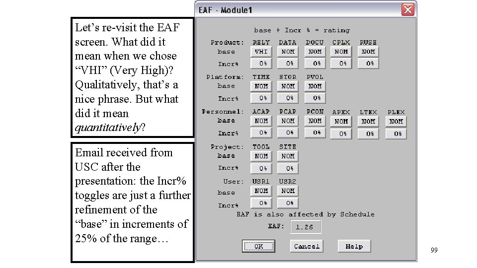
This screen will popup. As you click on any given button top row button, the button’s title will change (Nom, High, Very Low, etc) AND you will see the EAF at the bottom of the screen change. 94

I have changed ONLY the button for RELY to VHI and by doing so, the EAF has changed to 1. 26. So we just increased the Effort equation by 26%!!! Click OK to see the result. 95

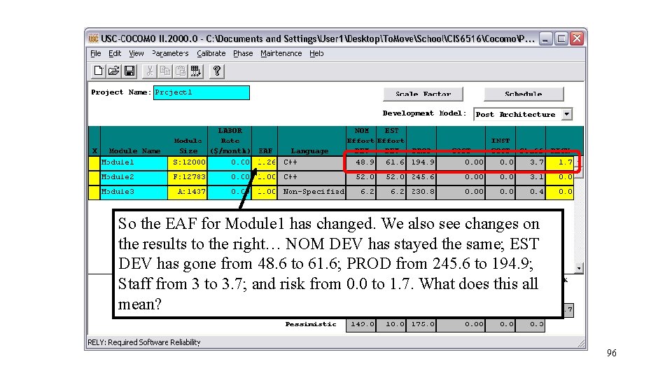
So the EAF for Module 1 has changed. We also see changes on the results to the right… NOM DEV has stayed the same; EST DEV has gone from 48. 6 to 61. 6; PROD from 245. 6 to 194. 9; Staff from 3 to 3. 7; and risk from 0. 0 to 1. 7. What does this all mean? 96

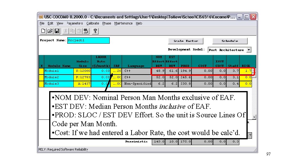
• NOM DEV: Nominal Person Man Months exclusive of EAF. • EST DEV: Median Person Months inclusive of EAF. • PROD: SLOC / EST DEV Effort. So the unit is Source Lines Of Code per Man Month. • Cost: If we had entered a Labor Rate, the cost would be calc’d. 97

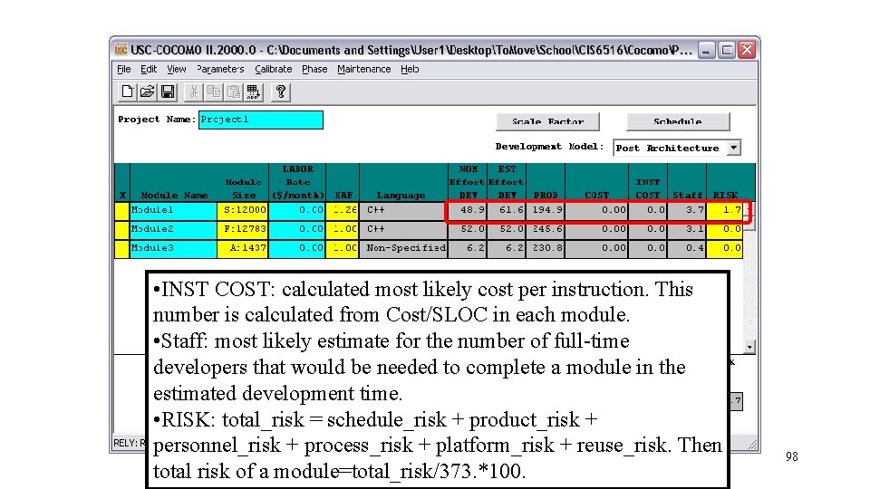
• INST COST: calculated most likely cost per instruction. This number is calculated from Cost/SLOC in each module. • Staff: most likely estimate for the number of full-time developers that would be needed to complete a module in the estimated development time. • RISK: total_risk = schedule_risk + product_risk + personnel_risk + process_risk + platform_risk + reuse_risk. Then total risk of a module=total_risk/373. *100. 98

Let’s re-visit the EAF screen. What did it mean when we chose “VHI” (Very High)? Qualitatively, that’s a nice phrase. But what did it mean quantitatively? Email received from USC after the presentation: the Incr% toggles are just a further refinement of the “base” in increments of 25% of the range… 99

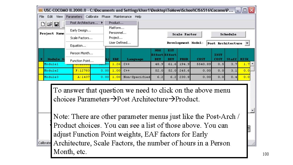
To answer that question we need to click on the above menu choices Parameters Post Architecture Product. Note: There are other parameter menus just like the Post-Arch / Product choices. You can see a list of those above. You can adjust Function Point weights, EAF factors for Early Architecture, Scale Factors, the number of hours in a Person Month, etc. 100

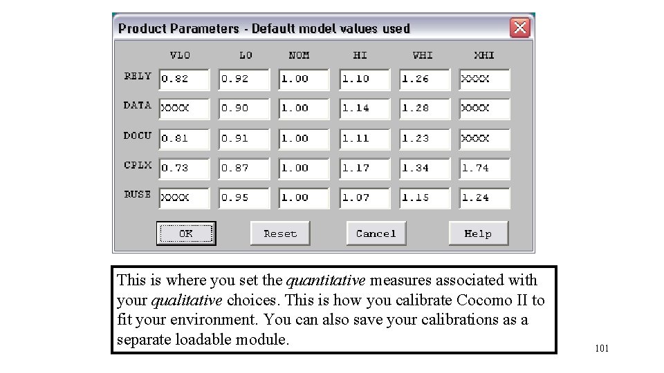
This is where you set the quantitative measures associated with your qualitative choices. This is how you calibrate Cocomo II to fit your environment. You can also save your calibrations as a separate loadable module. 101

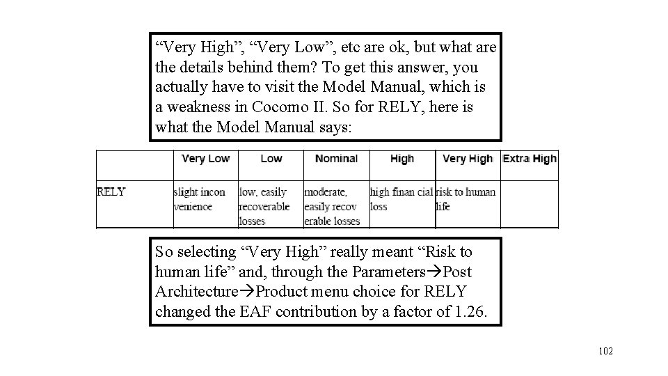
“Very High”, “Very Low”, etc are ok, but what are the details behind them? To get this answer, you actually have to visit the Model Manual, which is a weakness in Cocomo II. So for RELY, here is what the Model Manual says: So selecting “Very High” really meant “Risk to human life” and, through the Parameters Post Architecture Product menu choice for RELY changed the EAF contribution by a factor of 1. 26. 102

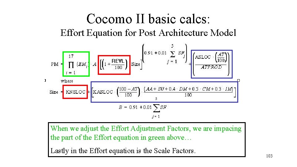
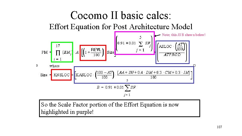
Cocomo II basic calcs: Effort Equation for Post Architecture Model When we adjust the Effort Adjustment Factors, we are impacing the part of the Effort equation in green above… Lastly in the Effort equation is the Scale Factors. 103

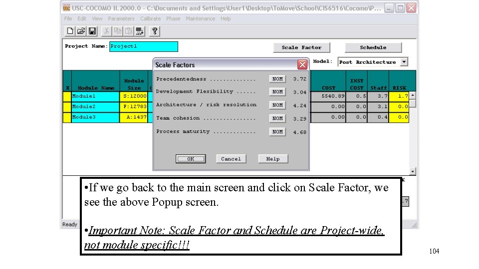
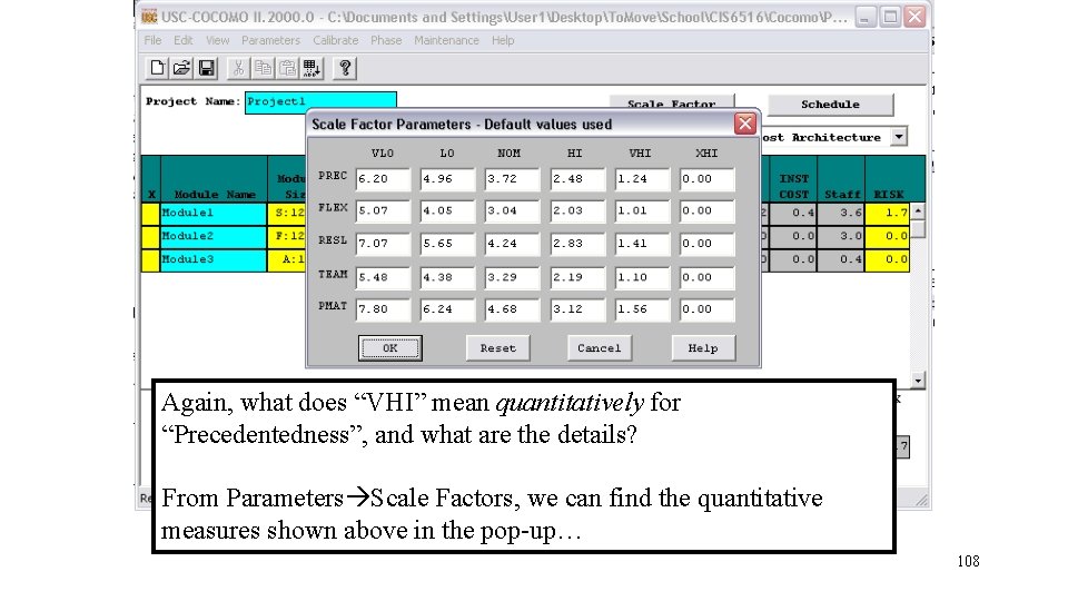
• If we go back to the main screen and click on Scale Factor, we see the above Popup screen. • Important Note: Scale Factor and Schedule are Project-wide, not module specific!!! 104

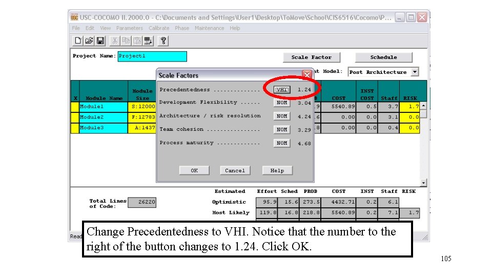
Change Precedentedness to VHI. Notice that the number to the right of the button changes to 1. 24. Click OK. 105

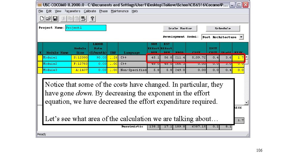
Notice that some of the costs have changed. In particular, they have gone down. By decreasing the exponent in the effort equation, we have decreased the effort expenditure required. Let’s see what area of the calculation we are talking about… 106

Cocomo II basic calcs: Effort Equation for Post Architecture Model Note; this IS B shown below! So the Scale Factor portion of the Effort Equation is now highlighted in purple! 107

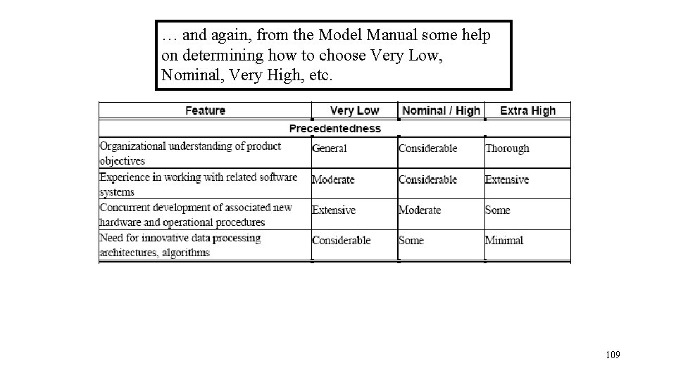
Again, what does “VHI” mean quantitatively for “Precedentedness”, and what are the details? From Parameters Scale Factors, we can find the quantitative measures shown above in the pop-up… 108

… and again, from the Model Manual some help on determining how to choose Very Low, Nominal, Very High, etc. 109

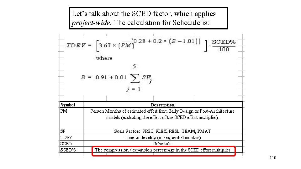
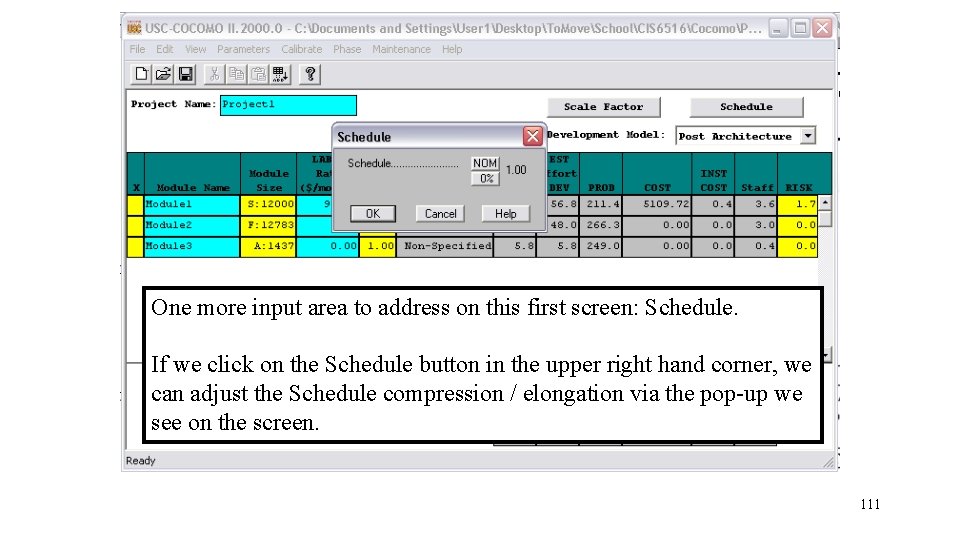
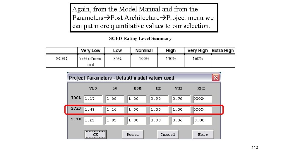
Let’s talk about the SCED factor, which applies project-wide. The calculation for Schedule is: 110

One more input area to address on this first screen: Schedule. If we click on the Schedule button in the upper right hand corner, we can adjust the Schedule compression / elongation via the pop-up we see on the screen. 111

Again, from the Model Manual and from the Parameters Post Architecture Project menu we can put more quantitative values to our selection. 112

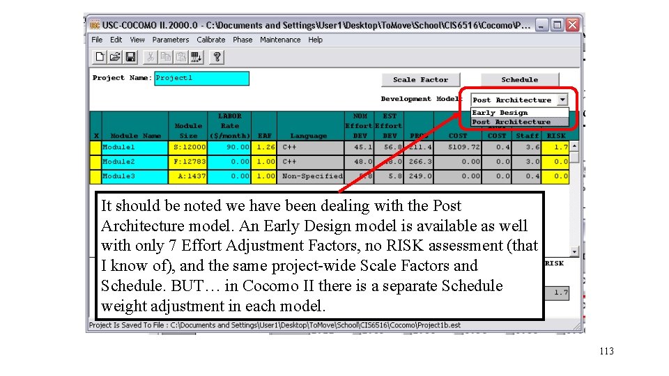
It should be noted we have been dealing with the Post Architecture model. An Early Design model is available as well with only 7 Effort Adjustment Factors, no RISK assessment (that I know of), and the same project-wide Scale Factors and Schedule. BUT… in Cocomo II there is a separate Schedule weight adjustment in each model. 113

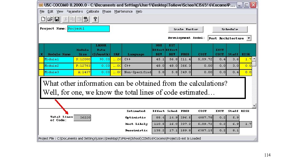
What other information can be obtained from the calculations? Well, for one, we know the total lines of code estimated… 114

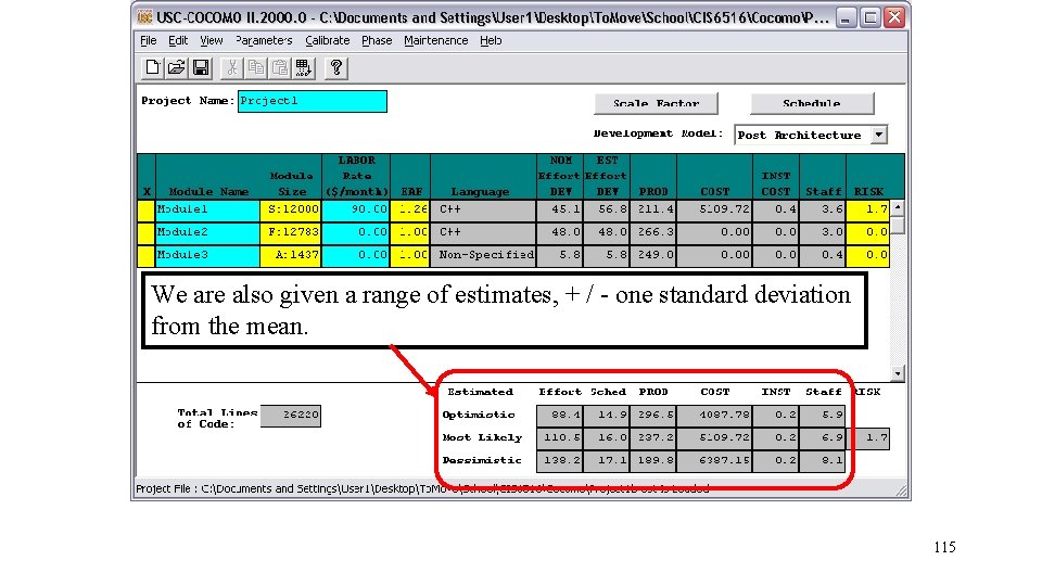
We are also given a range of estimates, + / - one standard deviation from the mean. 115

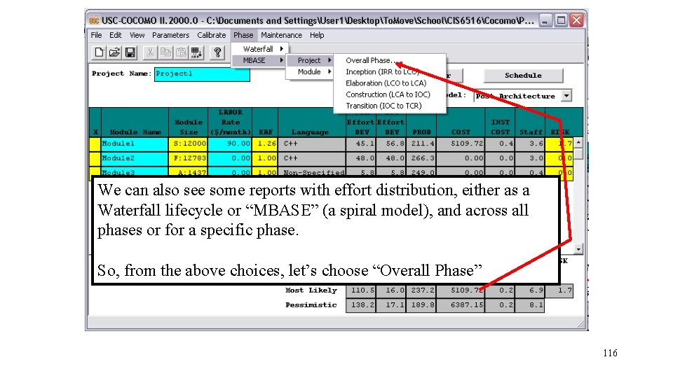
We can also see some reports with effort distribution, either as a Waterfall lifecycle or “MBASE” (a spiral model), and across all phases or for a specific phase. So, from the above choices, let’s choose “Overall Phase” 116

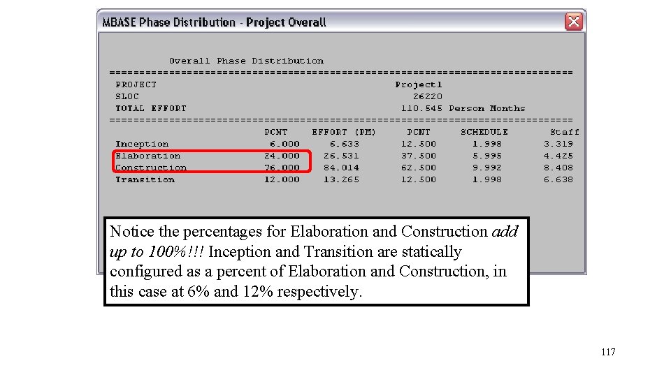
Notice the percentages for Elaboration and Construction add up to 100%!!! Inception and Transition are statically configured as a percent of Elaboration and Construction, in this case at 6% and 12% respectively. 117

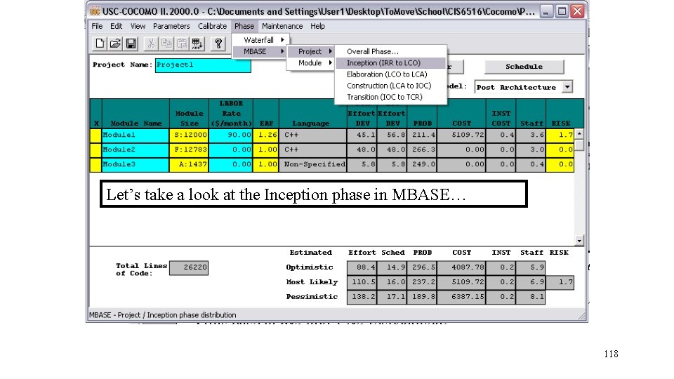
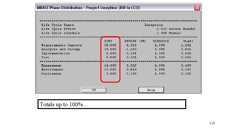
Let’s take a look at the Inception phase in MBASE… 118

Totals up to 100%… 119

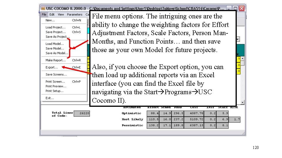
File menu options. The intriguing ones are the ability to change the weighting factors for Effort Adjustment Factors, Scale Factors, Person Man. Months, and Function Points… and then save those as your own Model for future projects. Also, if you choose the Export option, you can then load up additional reports via an Excel interface (you can find the Excel file by navigating via the Start Programs USC Cocomo II). 120

Parting thoughts… 1. There are limited online calculator versions of Cocomo 81 and Cocomo II: http: //sunset. usc. edu/research/COCOMOII/cocomo 81_pgm/cocomo 81. html http: //sunset. usc. edu/research/COCOMOII/expert_cocomo 2000. html 2. Soft. Star. Systems. com sells Co. Star, a Cocomo II on steroids. A trial version limited to 5, 000 lines of code is available. Single user license starts at $2, 000!!! 3. It’s really hard getting a good handle on all the current algorithms for Cocomo II. It varies over time, administered by fluctuating grad students, etc. 4. Home website for Cocomo: http: //sunset. usc. edu/csse/research/COCOMOII/cocomo_main. html 5. Email from USC student: There is no source code available for COCOMO II. This would be an interesting open source/thesis project if you could get their data! 121