Topic 8 Model Diagnostics Outline Diagnostics to check

Topic 8: Model Diagnostics

Outline • Diagnostics to check model assumptions – Diagnostics concerning X – Diagnostics using the residuals

Diagnostics and remedial measures • Diagnostics: look at the data to diagnose situations where the assumptions of our model are violated • Remedies: changes in analytic strategy to fix these problems

Look at the data • Before trying to describe the relationship between a response variable (Y) and an explanatory variable (X), we should look at the distributions of these variables • We should always look at X • If Y depends on X, looking at Y alone may not be very informative

Diagnostics for X • If X has many values, use Proc Univariate to get numerical summaries (e. g. , mean, median, quartiles) • If X has only a few values, use Proc Freq or the Freq option in Proc Univariate to get summaries (e. g. , percentages, counts)

Diagnostics for X • Examine the distribution of X – Is it skewed? – Are there outliers? • Do the values of X depend on time (i. e. , the order in which they were collected)?

What’s the concern? • Model estimates based on means and sums of squares • These numerical summaries are not robust to outliers • Can inflate variance or influence trend • Observations that show a pattern over time are not independent

Important Statistics • • • Mean Standard deviation Skewness Kurtosis Range

Example: Toluca lot size data toluca; infile ‘. . /data/CH 01 TA 01. txt'; input lotsize hours; seq=_n_; proc univariate data=toluca plot; var lotsize; run;

Crude Plots Stem 12 11 10 9 8 7 6 5 4 3 2 Leaf 0 00 00 000 000 00 0 ----+----+ Multiply Stem. Leaf by 10**+1 # 1 2 2 4 3 3 1 3 2 3 1 Boxplot | | | +-----+ | | *--+--* | | +-----+ | | |

Moments N 25 Sum Weights Mean 70 Sum Observations Std Deviation 28. 7228132 Variance Skewness -0. 1032081 Kurtosis Uncorrected SS 142300 Corrected SS Coeff Variation 41. 0325903 Std Error Mean 25 1750 825 -1. 0794107 19800 5. 74456265

Location and Spread Basic Statistical Measures Location Variability Mean 70. 00000 Std Deviation 28. 72281 Median 70. 00000 Variance 825. 00000 Mode 100. 00000 90. 00000 Range Interquartile Range 40. 00000

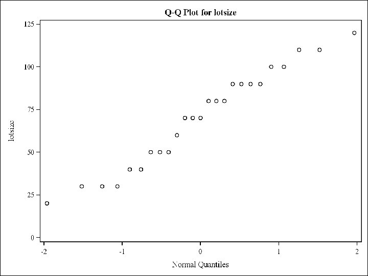
Quantiles (Definition 5) Quantile Estimate 100% Max 120 99% 120 95% 110 90% 110 75% Q 3 90 50% Median 70 25% Q 1 50 10% 30 5% 30 1% 20 0% Min 20

Extreme Observations Lowest Highest Value 20 Obs 14 Value 100 Obs 9 30 21 100 16 30 17 110 15 30 2 110 20 40 23 120 7

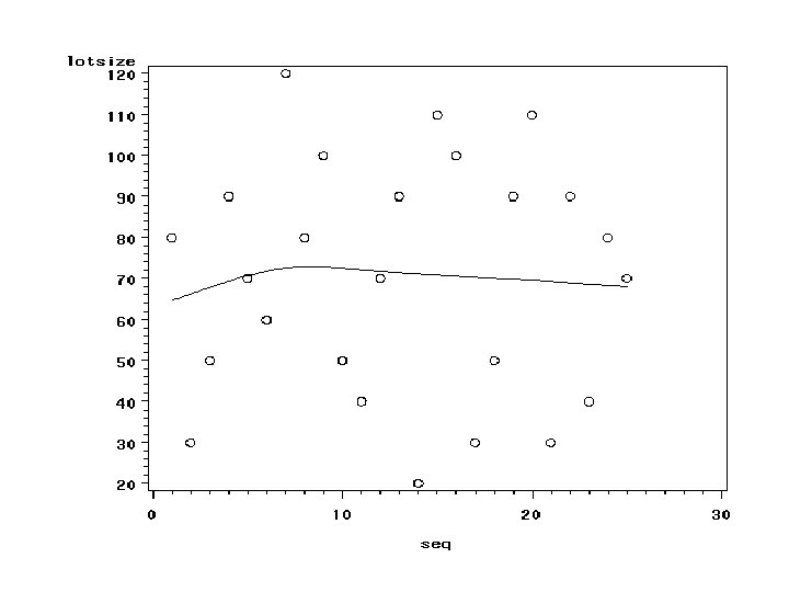
SAS CODE FOR “TREND IN ORDER? ” symbol 1 v=circle i=sm 70; proc gplot data=a 1; plot lotsize*seq; run;

Normal distributions • Our model does not state that X comes from a single normal population • Same comment applies to Y • In some cases, X and/or Y may be normal and it can be useful to know this

Normal quantile plots • Consider n=5 observations iid N(0, 1) • From Table B. 1, we find – P(z -. 84) =. 20 – P(-. 84 < z -. 25) =. 20 – P(-. 25 < z . 25) =. 20 – P(. 25 < z . 84) =. 20 – P(z >. 84) =. 20

Normal quantile plots • So we expect – One observation -. 84 – One observation in (-. 84, -. 25) – One observation in (-. 25, . 25) – One observation in (25, . 84) – One observation >. 84

Normal quantile plots • Zi = -1((i-. 375)/(n+. 25)), i=1 to n • Plot the order statistics X(i) vs Zi • KNNL plots X(i) vs s Zi • Doesn’t affect nature of plot

Normal quantile plots • The standardized X variable is z = (X - μ)/σ • So, X = μ + σ z • If the data are approximately normal, the relationship will be approximately linear with slope close to σ and intercept close to μ.

SAS CODE proc univariate data=toluca plot; var lotsize; qqplot lotsize; run;

Diagnostics for residuals • • • Model: Yi = β 0 + β 1 Xi + ei Predicted values: Ŷi = b 0 + b 1 Xi Residuals: ei = Yi – Ŷi So, Yi = Ŷi + ei The ei should be similar to the ei The model assumes ei iid N(0, σ2)

Plot PLOT Plot

Questions addressed by diagnostics for residuals • • • Is the relationship linear? Does the variance depend on X? Are there outliers? Do the errors depend on order? Are the errors normal? Are the errors dependent?

Is the Relationship Linear? • Plot Y vs X • Plot e vs X (residual plot) • Residual plot better emphasizes deviations from linear pattern

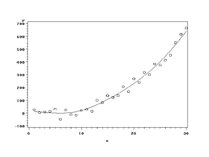
SAS CODE: Fake #1 libname xxx ‘. . /data’; Data xxx. a 100; do x=1 to 30; y=x*x-10*x+30+25*normal(0); output; end; run; Generates data set where Y=X 2 -10 X+30 Errors are normally distributed with s=25

SAS CODE proc reg data=xxx. a 100; model y=x; output out=a 2 r=resid; run;

OUTPUT Source Model Error Corrected Total Variable Intercept x DF 1 1 Analysis of Variance Sum of Mean DF Squares Square F Value Pr > F 1 1032098 170. 95 <. 0001 28 169048 6037. 41596 29 1201145 Parameter Estimates Parameter Standard Estimate Error t Value Pr > |t| -145. 37495 29. 09684 -5. 00 <. 0001 21. 42943 1. 63899 13. 07 <. 0001 A significant positive relationship!!

SAS CODE: Visual Checks symbol 1 v=circle i=rl; proc gplot data=a 2; plot y*x; Scatterplot with regression line run; symbol 1 v=circle i=sm 60; proc gplot data=a 2; Scatterplot with smoothed curve plot y*x; proc gplot data=a 2; Residual plot resid*x/ vref=0; run;

Does not appear to be linear

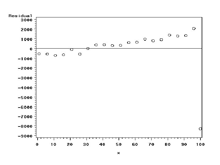
Nonlinear behavior easier to see here? !

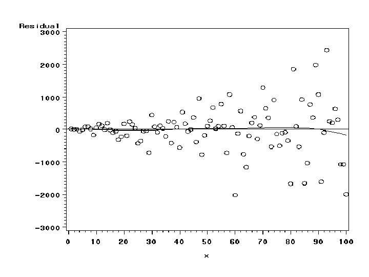
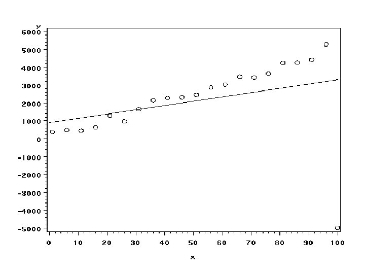
Does the variance depend on X? • Plot Y vs X • Plot e vs X • Plot of e vs X will emphasize problems with the variance assumption

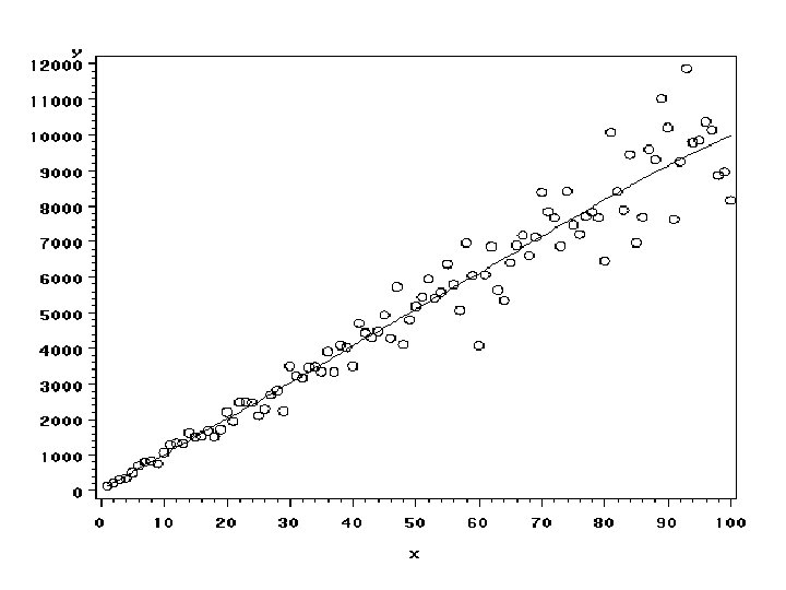
SAS CODE: Fake #2 libname xxx ‘. . /data'; Data xxx. a 100 a; do x=1 to 100; y=30+100*x+10*x*normal(0); output; end; run; Generates data set where Y=30 + 100 X Errors are normally distributed with s=10 X

SAS CODE proc reg data=xxx. a 100 a; model y=x; output out=a 2 r=resid; run;

OUTPUT Source Model Error Corrected Total Variable Intercept x Analysis of Variance Sum of Mean DF Squares Square F Value Pr > F 1 856723171 1682. 55 <. 0001 98 49899722 509181 99 906622893 Parameter Estimates Parameter Standard DF Estimate Error t Value Pr > |t| 1 13. 80557 143. 79092 0. 10 0. 9237 1 101. 39875 2. 47200 41. 02 <. 0001 A significant positive relationship!!

SAS CODE: Visual Checks symbol 1 v=circle i=sm 60; proc gplot data=a 2; Scatterplot with plot y*x; smoothed curve proc gplot data=a 2; Residual plot resid*x / vref=0; run;

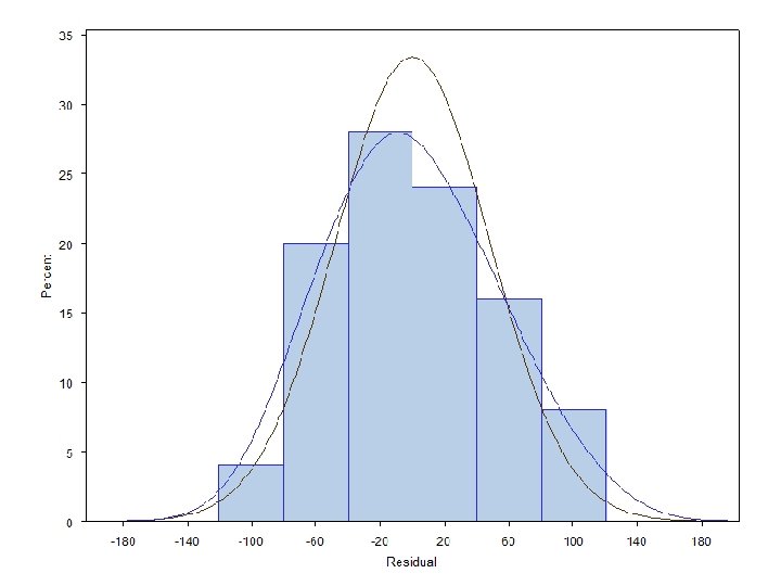
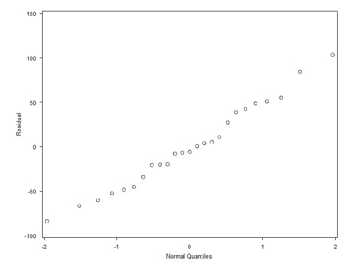
Are the errors normal? • The real question is whether the distribution of the errors is far enough away from normal to invalidate our confidence intervals and significance tests • Look at the residuals’ distribution • Use a normal quantile plot

SAS CODE data a 1; infile ‘. . dataCH 01 TA 01. txt'; input lotsize hours; proc reg data=a 1; model hours=lotsize; output out=a 2 r=resid; proc univariate data=a 2 plot normal; var resid; histogram resid / normal kernel; qqplot resid;

Univariate Output Fitted Normal Distribution for resid Parameters for Normal Distribution Parameter Symbol Estimate Mean Mu 0 Std Dev Sigma 47. 79534 Goodness-of-Fit Tests for Normal Distribution Test Kolmogorov-Smirnov Cramer-von Mises Anderson-Darling ----Statistic----D 0. 09571960 W-Sq 0. 03326349 A-Sq 0. 20714170 ------p Value-----Pr > D >0. 150 Pr > W-Sq >0. 250 Pr > A-Sq >0. 250 No obvious deviations from normality as P -values are greater than 0. 05

Dependent Errors • Usually we see this in a plot of residuals vs time order (KNNL) or seq (our SAS variable) • We can have trends and/or cyclical effects in the residuals • If you are interested read KNNL pg 108 -110

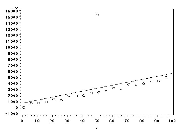
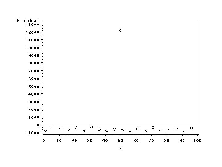
Are there outliers? • Plot Y vs X • Plot e vs X • Plot of e vs X should emphasize an outlier

SAS CODE: Fake #3 Data xxx. a 100 b 1; do x=1 to 100 by 5; y=30+50*x+200*normal(0); output; end; x=50; y=30+50*50+10000; d='out'; output; run; Generates data set where Y=30+50 X Errors are normally distributed with s=200

SAS CODE proc reg data=xxx. a 100 b 1; model y=x; where d ne 'out'; run; proc reg data=xxx. a 100 b 1; model y=x; output out=a 2 r=resid; run;

Without Outlier Source Model Error Corrected Total Variable Intercept x Analysis of Variance Sum of Mean DF Squares Square 1 42426770 18 853668 47426 19 43280438 F Value Pr > F 894. 59 <. 0001 Parameter Estimates Parameter Standard DF Estimate Error t Value Pr > |t| 1 -2. 54677 95. 29715 -0. 03 0. 9790 1 50. 51719 1. 68899 29. 91 <. 0001 s=217. 8

With Outlier Source Model Error Corrected Total Variable Intercept x Analysis of Variance Sum of Mean DF Squares Square 1 43888843 19 96206895 5063521 20 140095738 F Value 8. 67 Parameter Estimates Parameter Standard DF Estimate Error t Value Pr > |t| 1 432. 20263 979. 57661 0. 44 0. 6640 1 51. 37694 17. 45089 2. 94 0. 0083 Pr > F 0. 0083 s=2250. 2

SAS CODE: Visual Checks symbol 1 v=circle i=rl; proc gplot data=a 2; plot y*x; proc gplot data=a 2; plot resid*x/ vref=0; run;

Different kinds of outliers • The outlier in the last example influenced the intercept but not the slope • It inflated all of our standard errors • Here is an example of an outlier that influences the slope

SAS CODE Data xxx. a 100 c 1; do x=1 to 100 by 5; y=30+50*x+200*normal(0); output; end; x=100; y=30+50*100 -10000; d='out'; output; run;

SAS CODE proc reg data=xxx. a 100 c 1; model y=x; where d ne 'out'; run; proc reg data=xxx. a 100 c 1; model y=x; output out=a 2 r=resid; run;

Without Outlier Source Model Error Corrected Total Variable Intercept x Analysis of Variance Sum of Mean DF Squares Square 1 41233447 18 823612 45756 19 42057060 F Value Pr > F 901. 15 <. 0001 Parameter Estimates Parameter Standard DF Estimate Error t Value Pr > |t| 1 73. 28061 93. 60451 0. 78 0. 4439 1 49. 80168 1. 65899 30. 02 <. 0001

With Outlier Source Model Error Corrected Total Variable Intercept x Analysis of Variance Sum of Mean DF Squares Square 1 11151297 19 83888277 4415172 20 95039574 F Value 2. 53 Parameter Estimates Parameter Standard DF Estimate Error t Value Pr > |t| 1 903. 97793 899. 32018 1. 01 0. 3274 1 24. 13057 15. 18374 1. 59 0. 1285 Pr > F 0. 1285

SAS CODE: Visual Checks symbol 1 v=circle i=rl; proc gplot data=a 2; plot y*x; proc gplot data=a 2; plot resid*x/ vref=0; run;

Background Reading • Program topic 8. sas has code for the proc univariate diagnostics of X • Program residualchecks. sas have the residual analysis • The permanent sas data sets are a 100. sas 7 bdat, a 100 a. sas 7 bdat, a 100 b 1. sas 7 bdat, and a 100 c 1. sas 7 bdat. • Read sections 3. 8 and 3. 9