Topic 6 Relational Database Design CPS 510 Database

Topic 6 Relational Database Design CPS 510 Database Systems Abdolreza Abhari School of Computer Science Ryerson University 1

Topics in this Section • • Problems with bad database design Concept of decomposition Functional dependencies Normalization theory * Normal forms (BCNF and 3 NF) * Deriving normal forms • Multivalued dependnecies * 4 NF 2

Introduction • When designing a relational database schema * Several schemas are possible » Some are better and convenient » Some are bad and not desirable • Database design process involves selecting an appropriate schema * Uses the concept of data dependency » Simple functional dependency Student. No Student. Name » More complex multivalued dependency * Data dependencies obtain semantic information from the application 3

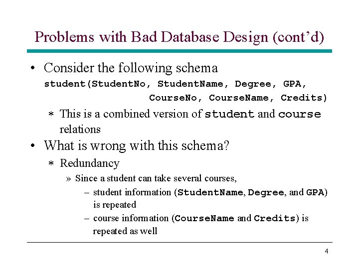
Problems with Bad Database Design (cont’d) • Consider the following schema student(Student. No, Student. Name, Degree, GPA, Course. No, Course. Name, Credits) * This is a combined version of student and course relations • What is wrong with this schema? * Redundancy » Since a student can take several courses, – student information (Student. Name, Degree, and GPA) is repeated – course information (Course. Name and Credits) is repeated as well 4

Problems with Bad Database Design (cont’d) * Update anomalies » Direct consequence of redundancy » We could update the GPA in one tuple while leaving as is in other tuples for the same student * Insertion anomalies » We cannot insert a new course unless at least one student is taking it » Could use NULL values but introduce problems of their own – In general, use NULL values only when unavoidable * Deletion anomalies » Inverse of the last problem » If we delete all students taking a course, we also lose unintentionally information on the course 5

Decomposition • What is the solution? * Split the relation into two or more relations » This process is called decomposition » We can use join to get back the original information » The whole theory of relational database design deals with how to do this decomposition so that the resulting schema satisfies desirable properties * Decomposition can also lead to problems if not done properly student(Student. No, Student. Name, Degree, GPA) course(Course. No, Course. Name, Credits, Degree) » This leads to loss of information (spurious tuples) when joined 6

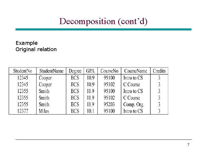
Decomposition (cont’d) Example Original relation 7

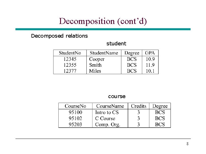
Decomposition (cont’d) Decomposed relations student course 8

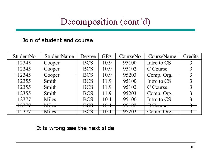
Decomposition (cont’d) Join of student and course It is wrong see the next slide 9

Decomposition (cont’d) * The join of student and course generates 3 spurious tuples * A good decomposition should be lossless or nonadditive join property – Ensures that no spurious tuples are generated when a natural join is applied to the relations in the decomposition 10

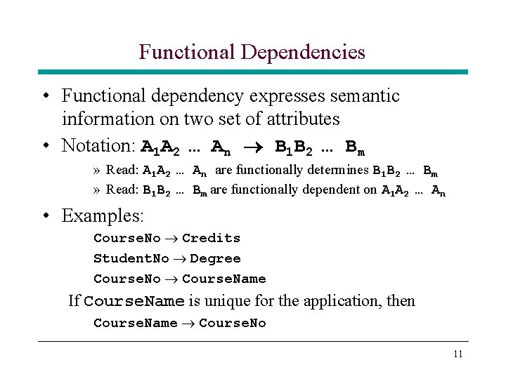
Functional Dependencies • Functional dependency expresses semantic information on two set of attributes • Notation: A 1 A 2 … An B 1 B 2 … Bm » Read: A 1 A 2 … An are functionally determines B 1 B 2 … Bm » Read: B 1 B 2 … Bm are functionally dependent on A 1 A 2 … An • Examples: Course. No Credits Student. No Degree Course. No Course. Name If Course. Name is unique for the application, then Course. Name Course. No 11

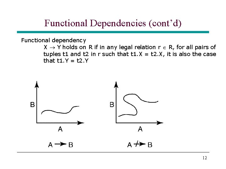
Functional Dependencies (cont’d) Functional dependency X Y holds on R if in any legal relation r R, for all pairs of tuples t 1 and t 2 in r such that t 1. X = t 2. X, it is also the case that t 1. Y = t 2. Y 12

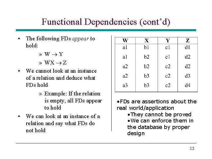
Functional Dependencies (cont’d) • The following FDs appear to hold: » W Y » WX Z • We cannot look at an instance of a relation and deduce what FDs hold » Example: If the relation is empty, all FDs appear to hold • We can look at an instance of a relation and say what FDs do not hold • FDs are assertions about the real world/application • They cannot be proved • We can enforce them in the database by proper design 13

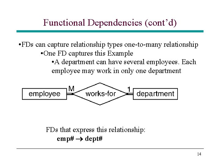
Functional Dependencies (cont’d) • FDs can capture relationship types one-to-many relationship • One FD captures this Example • A department can have several employees. Each employee may work in only one department FDs that express this relationship: emp# dept# 14

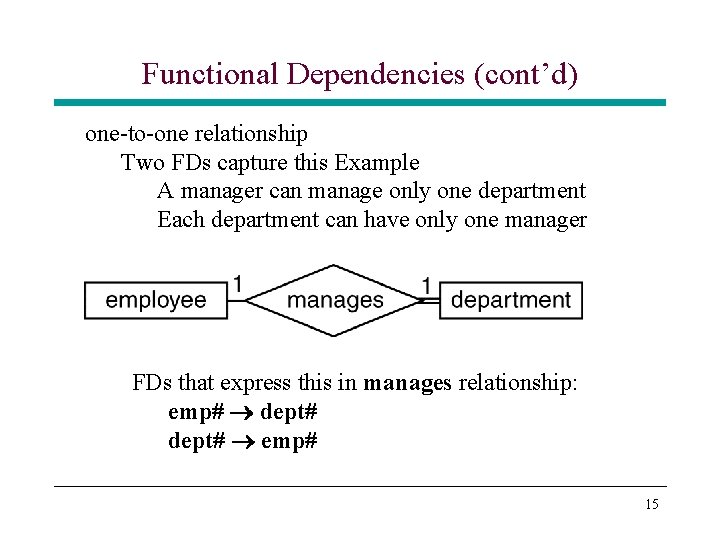
Functional Dependencies (cont’d) one-to-one relationship Two FDs capture this Example A manager can manage only one department Each department can have only one manager FDs that express this in manages relationship: emp# dept# emp# 15

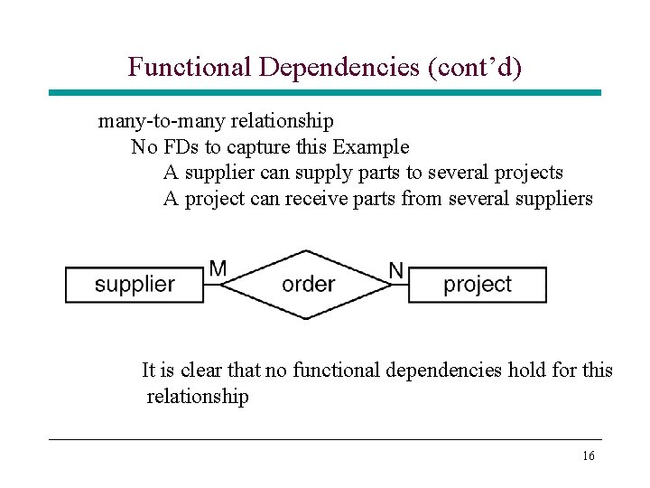
Functional Dependencies (cont’d) many-to-many relationship No FDs to capture this Example A supplier can supply parts to several projects A project can receive parts from several suppliers It is clear that no functional dependencies hold for this relationship 16

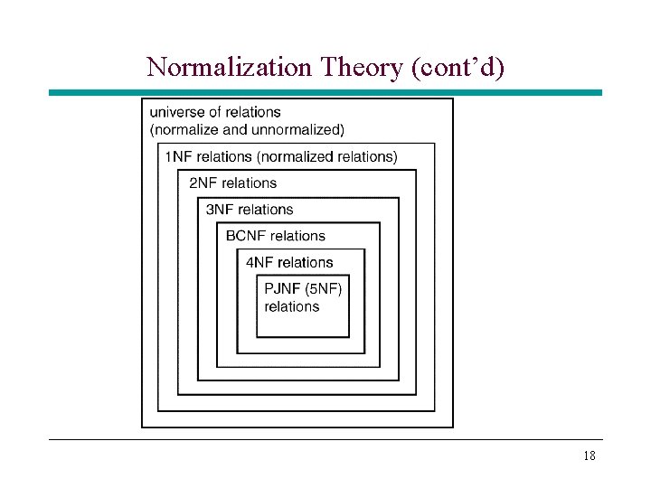
Normalization Theory • Normalization theory is built around the concept of normal forms » A relation is said to be in a normal if it satisfies a certain set of specified constraints • Several normal forms have been defined * 1 NF, 2 NF, 3 NF, BCNF » Based on functional dependency concept * 4 NF » Based on multivalued dependencies * 5 NF, … • In practical terms, focus is on BCNF/3 NF designs 17

Normalization Theory (cont’d) 18

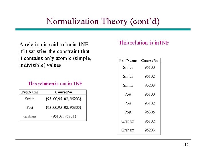
Normalization Theory (cont’d) A relation is said to be in 1 NF if it satisfies the constraint that it contains only atomic (simple, indivisible) values This relation is in 1 NF This relation is not in 1 NF 19

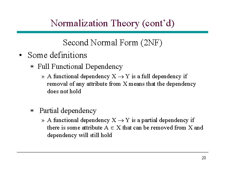
Normalization Theory (cont’d) Second Normal Form (2 NF) • Some definitions * Full Functional Dependency » A functional dependency X Y is a full dependency if removal of any attribute from X means that the dependency does not hold * Partial dependency » A functional dependency X Y is a partial dependency if there is some attribute A X that can be removed from X and dependency will still hold 20

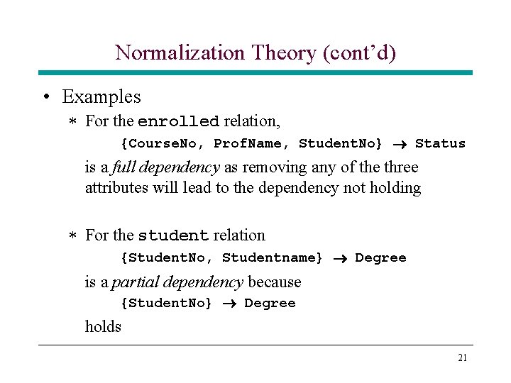
Normalization Theory (cont’d) • Examples * For the enrolled relation, {Course. No, Prof. Name, Student. No} Status is a full dependency as removing any of the three attributes will lead to the dependency not holding * For the student relation {Student. No, Studentname} Degree is a partial dependency because {Student. No} Degree holds 21

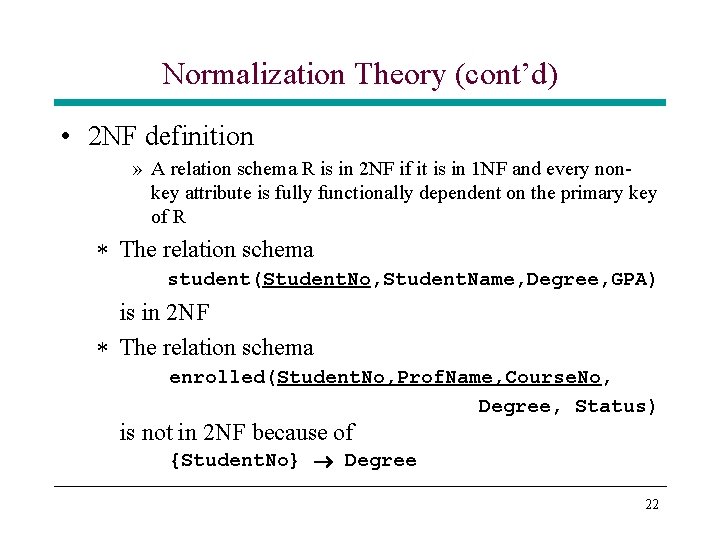
Normalization Theory (cont’d) • 2 NF definition » A relation schema R is in 2 NF if it is in 1 NF and every nonkey attribute is fully functionally dependent on the primary key of R * The relation schema student(Student. No, Student. Name, Degree, GPA) is in 2 NF * The relation schema enrolled(Student. No, Prof. Name, Course. No, Degree, Status) is not in 2 NF because of {Student. No} Degree 22

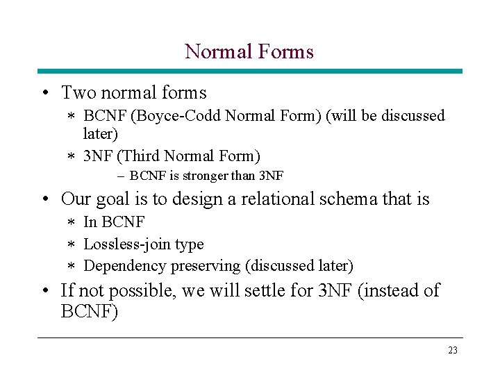
Normal Forms • Two normal forms * BCNF (Boyce-Codd Normal Form) (will be discussed later) * 3 NF (Third Normal Form) – BCNF is stronger than 3 NF • Our goal is to design a relational schema that is * In BCNF * Lossless-join type * Dependency preserving (discussed later) • If not possible, we will settle for 3 NF (instead of BCNF) 23

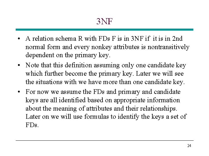
3 NF • A relation schema R with FDs F is in 3 NF if it is in 2 nd normal form and every nonkey attributes is nontransitively dependent on the primary key. • Note that this definition assuming only one candidate key which further become the primary key. Later we will see the situations with we have more than one candidate key. • For now we assume the FDs and primary and candidate keys are all identified based on appropriate information about the meaning of attributes and their relationships. Later on we will use formulas to identify the keys a set of FDs. 24

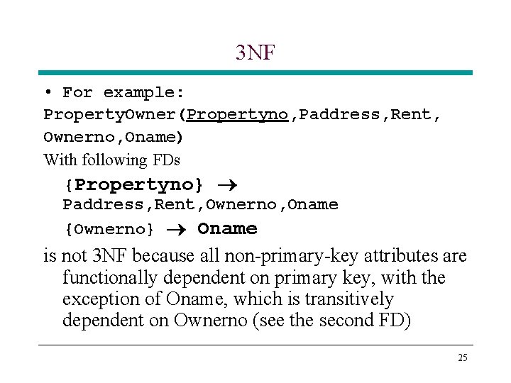
3 NF • For example: Property. Owner(Propertyno, Paddress, Rent, Ownerno, Oname) With following FDs {Propertyno} Paddress, Rent, Ownerno, Oname {Ownerno} Oname is not 3 NF because all non-primary-key attributes are functionally dependent on primary key, with the exception of Oname, which is transitively dependent on Ownerno (see the second FD) 25

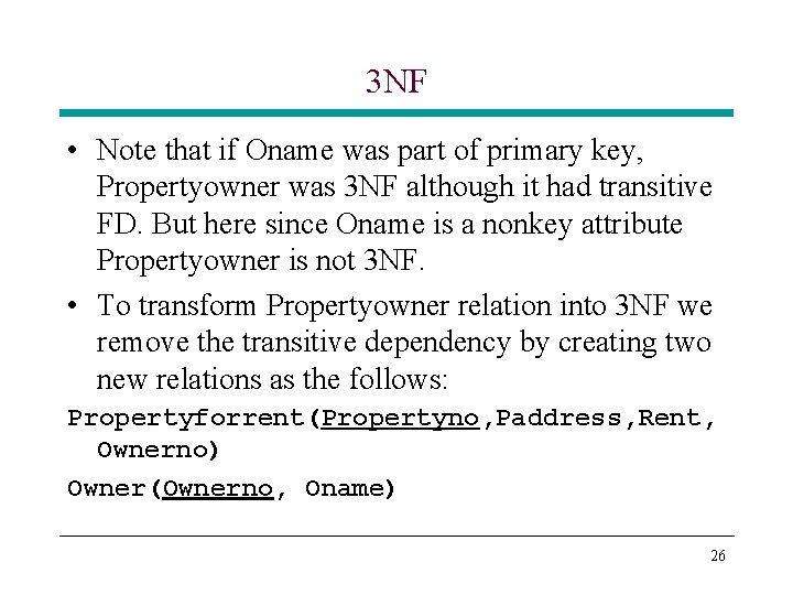
3 NF • Note that if Oname was part of primary key, Propertyowner was 3 NF although it had transitive FD. But here since Oname is a nonkey attribute Propertyowner is not 3 NF. • To transform Propertyowner relation into 3 NF we remove the transitive dependency by creating two new relations as the follows: Propertyforrent(Propertyno, Paddress, Rent, Ownerno) Owner(Ownerno, Oname) 26

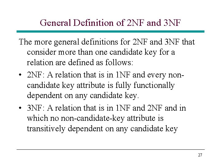
General Definition of 2 NF and 3 NF The more general definitions for 2 NF and 3 NF that consider more than one candidate key for a relation are defined as follows: • 2 NF: A relation that is in 1 NF and every noncandidate key attribute is fully functionally dependent on any candidate key. • 3 NF: A relation that is in 1 NF and 2 NF and in which no non-candidate-key attribute is transitively dependent on any candidate key 27

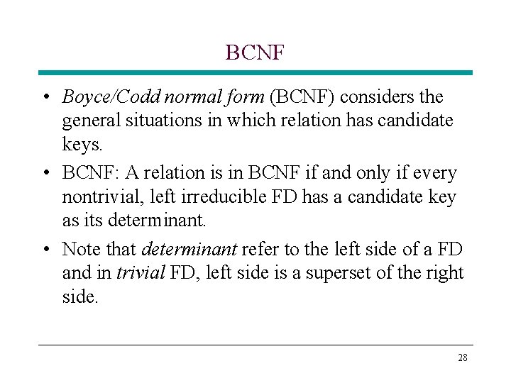
BCNF • Boyce/Codd normal form (BCNF) considers the general situations in which relation has candidate keys. • BCNF: A relation is in BCNF if and only if every nontrivial, left irreducible FD has a candidate key as its determinant. • Note that determinant refer to the left side of a FD and in trivial FD, left side is a superset of the right side. 28

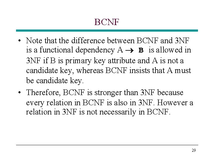
BCNF • Note that the difference between BCNF and 3 NF is a functional dependency A B is allowed in 3 NF if B is primary key attribute and A is not a candidate key, whereas BCNF insists that A must be candidate key. • Therefore, BCNF is stronger than 3 NF because every relation in BCNF is also in 3 NF. However a relation in 3 NF is not necessarily in BCNF. 29

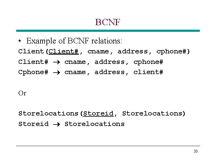
BCNF • Example of BCNF relations: Client(Client#, cname, address, cphone#) Client# cname, address, cphone# Cphone# cname, address, client# Or Storelocations(Storeid, Storelocations) Storeid Storelocations 30

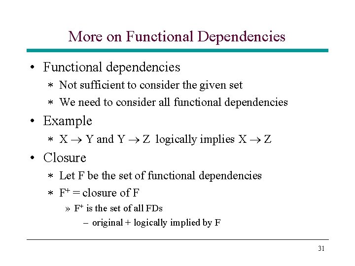
More on Functional Dependencies • Functional dependencies * Not sufficient to consider the given set * We need to consider all functional dependencies • Example * X Y and Y Z logically implies X Z • Closure * Let F be the set of functional dependencies * F+ = closure of F » F+ is the set of all FDs – original + logically implied by F 31

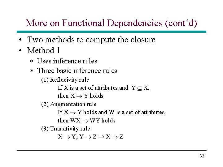
More on Functional Dependencies (cont’d) • Two methods to compute the closure • Method 1 * Uses inference rules * Three basic inference rules (1) Reflexivity rule If X is a set of attributes and Y X, then X Y holds (2) Augmentation rule If X Y holds and W is a set of attributes, then WX WY holds (3) Transitivity rule X Y, Y Z X Z 32

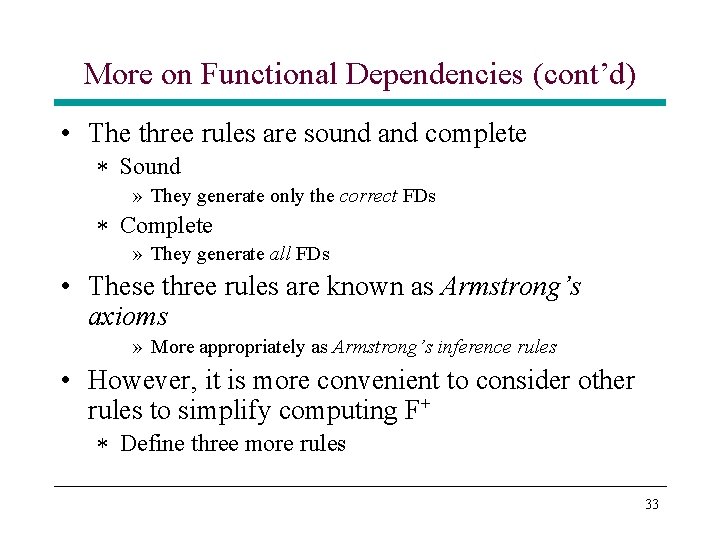
More on Functional Dependencies (cont’d) • The three rules are sound and complete * Sound » They generate only the correct FDs * Complete » They generate all FDs • These three rules are known as Armstrong’s axioms » More appropriately as Armstrong’s inference rules • However, it is more convenient to consider other rules to simplify computing F+ * Define three more rules 33

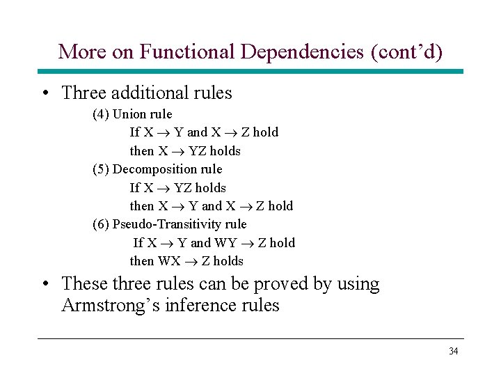
More on Functional Dependencies (cont’d) • Three additional rules (4) Union rule If X Y and X Z hold then X YZ holds (5) Decomposition rule If X YZ holds then X Y and X Z hold (6) Pseudo-Transitivity rule If X Y and WY Z hold then WX Z holds • These three rules can be proved by using Armstrong’s inference rules 34

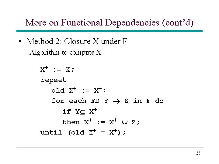
More on Functional Dependencies (cont’d) • Method 2: Closure X under F Algorithm to compute X+ X+ : = X; repeat old X+ : = X+; for each FD Y Z in F do if Y X+ then X+ : = X+ Z; until (old X+ = X+); 35

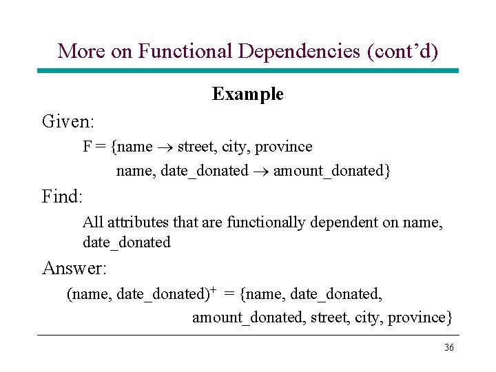
More on Functional Dependencies (cont’d) Example Given: F = {name street, city, province name, date_donated amount_donated} Find: All attributes that are functionally dependent on name, date_donated Answer: (name, date_donated)+ = {name, date_donated, amount_donated, street, city, province} 36

Desirable Properties of Decomposition • Two important properties * Lossless-join decomposition » Required for semantic correctness » When we join the decomposed relations, we should get back exact original relation contents – No spurious tuples * Dependency preservation » Required for efficiency » If checking a dependency requires joining two or more relations, it is very inefficient to enforce this FD. – Requires join when inserting a tuple 37

Finding Keys By FDs • We can define keys in terms of FDs • If R is a relation schema with » Attributes A 1, A 2, …, An » Functional dependencies F – X is a subset of A 1, A 2, …, An * X is a key if » X A 1, A 2, …, An is in F+, and » For no proper subset Y X Y A 1, A 2, …, An is in F+ * For a given relation schema, there may be several keys » There are called candidate keys » Primary key: Candidate key selected by the designer as the key 38

Finding Keys By FDs (cont’d) Example * Consider the relation schema R(C, S, P) with FDs {CS P, P C} * This schema has two candidate keys: {CS} and {SP} * {CS} is a candidate key because {CS}+ {C, S, P} * {SP} is a candidate key because {SP}+ {S, P, C} 39

Deriving 3 NF: Bernstein’s Algorithm • Derives 3 NF schema that is lossless and dependency preserving • Outline * There are 4 steps Step 1: – Find out facts about the real world QDifficult step but must be done in the design of a database QProbably takes more time than all the other steps put together – Result is a list of attributes and FDs 40

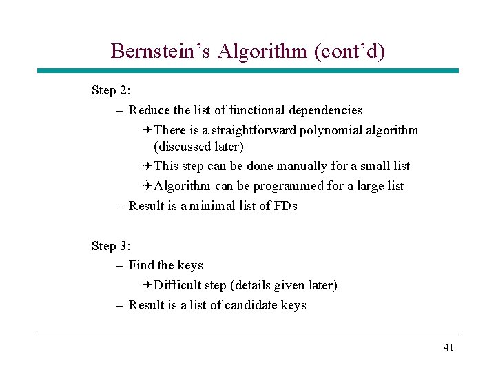
Bernstein’s Algorithm (cont’d) Step 2: – Reduce the list of functional dependencies QThere is a straightforward polynomial algorithm (discussed later) QThis step can be done manually for a small list QAlgorithm can be programmed for a large list – Result is a minimal list of FDs Step 3: – Find the keys QDifficult step (details given later) – Result is a list of candidate keys 41

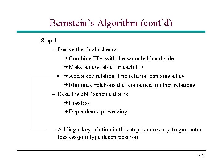
Bernstein’s Algorithm (cont’d) Step 4: – Derive the final schema QCombine FDs with the same left hand side QMake a new table for each FD QAdd a key relation if no relation contains a key QEliminate relations that contained in other relations – Result is 3 NF schema that is QLossless QDependency preserving – Adding a key relation in this step is necessary to guarantee lossless-join type decomposition 42

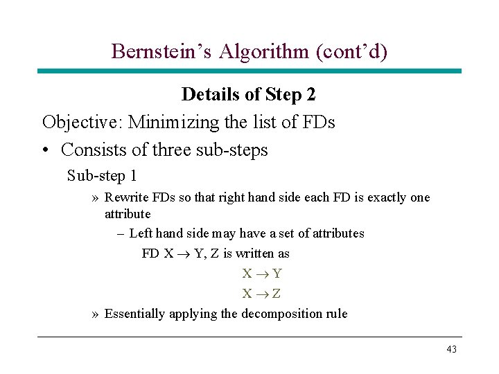
Bernstein’s Algorithm (cont’d) Details of Step 2 Objective: Minimizing the list of FDs • Consists of three sub-steps Sub-step 1 » Rewrite FDs so that right hand side each FD is exactly one attribute – Left hand side may have a set of attributes FD X Y, Z is written as X Y X Z » Essentially applying the decomposition rule 43

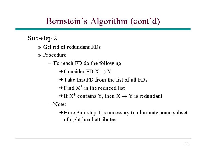
Bernstein’s Algorithm (cont’d) Sub-step 2 » Get rid of redundant FDs » Procedure – For each FD do the following QConsider FD X Y QTake this FD from the list of all FDs QFind X+ in the reduced list QIf X+ contains Y, then X Y is redundant – Note: QHere Sub-step 1 is necessary to eliminate some subset of right hand attributes 44

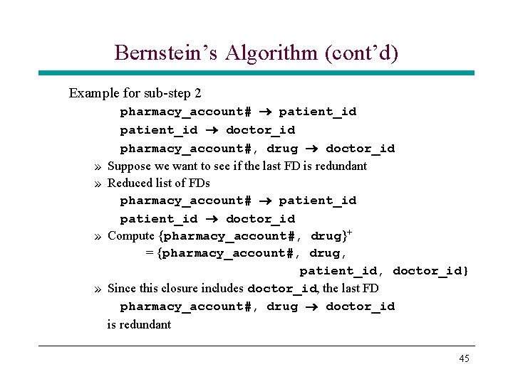
Bernstein’s Algorithm (cont’d) Example for sub-step 2 » » » » pharmacy_account# patient_id doctor_id pharmacy_account#, drug doctor_id Suppose we want to see if the last FD is redundant Reduced list of FDs pharmacy_account# patient_id doctor_id Compute {pharmacy_account#, drug}+ = {pharmacy_account#, drug, patient_id, doctor_id} Since this closure includes doctor_id, the last FD pharmacy_account#, drug doctor_id is redundant 45

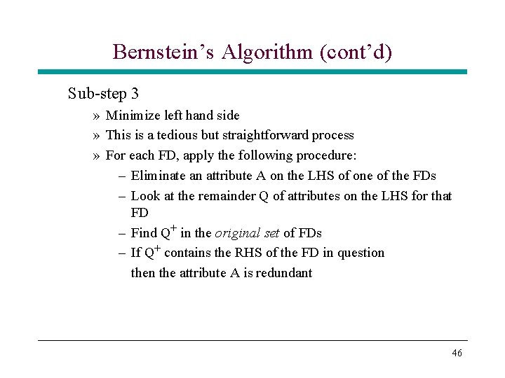
Bernstein’s Algorithm (cont’d) Sub-step 3 » Minimize left hand side » This is a tedious but straightforward process » For each FD, apply the following procedure: – Eliminate an attribute A on the LHS of one of the FDs – Look at the remainder Q of attributes on the LHS for that FD – Find Q+ in the original set of FDs – If Q+ contains the RHS of the FD in question the attribute A is redundant 46

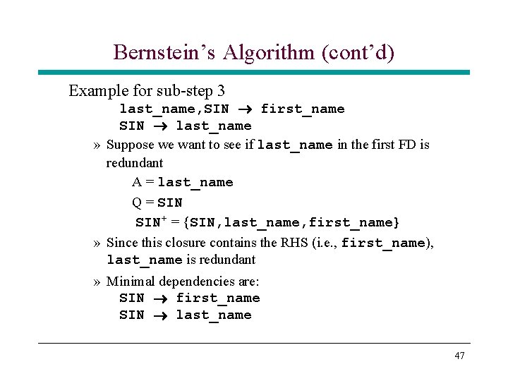
Bernstein’s Algorithm (cont’d) Example for sub-step 3 last_name, SIN first_name SIN last_name » Suppose we want to see if last_name in the first FD is redundant A = last_name Q = SIN+ = {SIN, last_name, first_name} » Since this closure contains the RHS (i. e. , first_name), last_name is redundant » Minimal dependencies are: SIN first_name SIN last_name 47

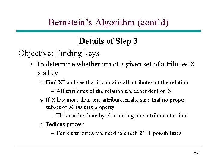
Bernstein’s Algorithm (cont’d) Details of Step 3 Objective: Finding keys * To determine whether or not a given set of attributes X is a key » Find X+ and see that it contains all attributes of the relation – All attributes of the relation are dependent on X » If X has more than one attribute, make sure that no proper subset of X has this property – This can be done by eliminating one attribute at a time » Tedious process – For k attributes, we need to check 2 k-1 possibilities 48

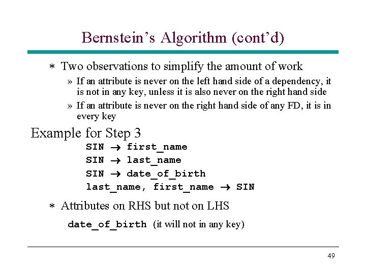
Bernstein’s Algorithm (cont’d) * Two observations to simplify the amount of work » If an attribute is never on the left hand side of a dependency, it is not in any key, unless it is also never on the right hand side » If an attribute is never on the right hand side of any FD, it is in every key Example for Step 3 SIN first_name SIN last_name SIN date_of_birth last_name, first_name SIN * Attributes on RHS but not on LHS date_of_birth (it will not in any key) 49

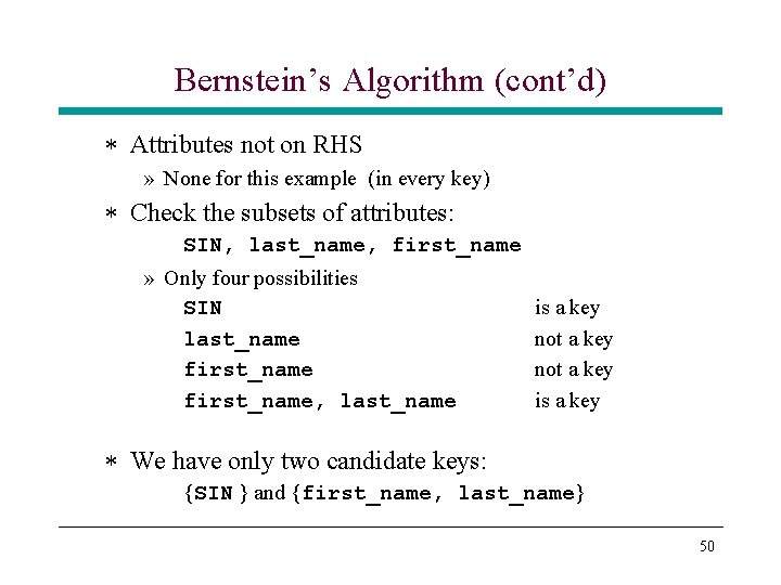
Bernstein’s Algorithm (cont’d) * Attributes not on RHS » None for this example (in every key) * Check the subsets of attributes: SIN, last_name, first_name » Only four possibilities SIN last_name first_name, last_name is a key not a key is a key * We have only two candidate keys: {SIN } and {first_name, last_name} 50

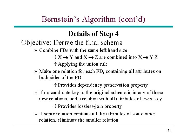
Bernstein’s Algorithm (cont’d) Details of Step 4 Objective: Derive the final schema » Combine FDs with the same left hand size QX Y and X Z are combined into X Y Z QApplying the union rule » Make one relation for each FD, containing all attributes on both sides of the FD QProvides dependency preservation property » If no candidate key to the original schema is in any of these new relations, add a relation with all attributes of some key QProvides lossless-join property » If some relation contains all the attributes of some other relation, eliminate the smaller relation 51

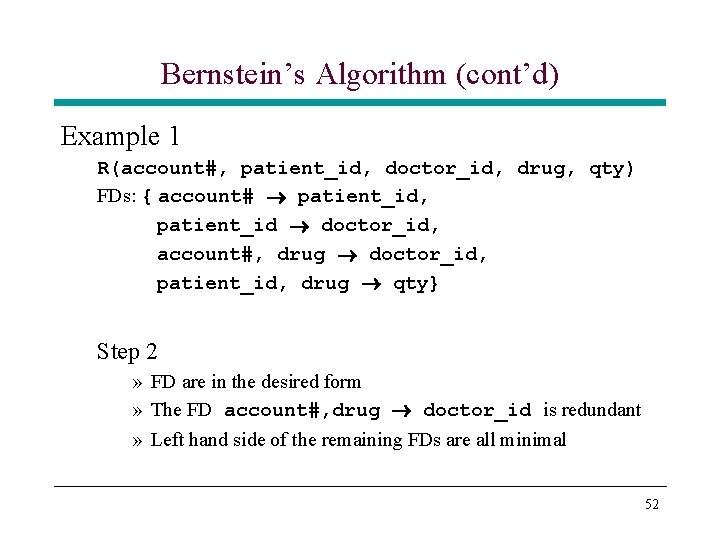
Bernstein’s Algorithm (cont’d) Example 1 R(account#, patient_id, doctor_id, drug, qty) FDs: { account# patient_id, patient_id doctor_id, account#, drug doctor_id, patient_id, drug qty} Step 2 » FD are in the desired form » The FD account#, drug doctor_id is redundant » Left hand side of the remaining FDs are all minimal 52

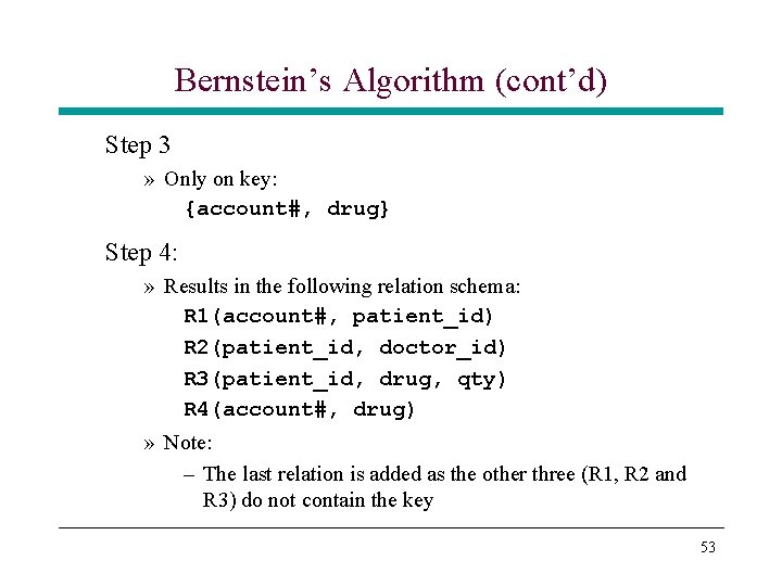
Bernstein’s Algorithm (cont’d) Step 3 » Only on key: {account#, drug} Step 4: » Results in the following relation schema: R 1(account#, patient_id) R 2(patient_id, doctor_id) R 3(patient_id, drug, qty) R 4(account#, drug) » Note: – The last relation is added as the other three (R 1, R 2 and R 3) do not contain the key 53

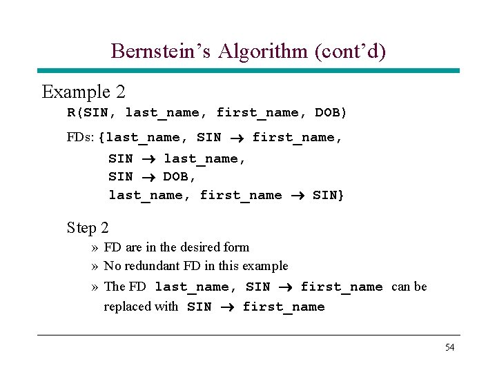
Bernstein’s Algorithm (cont’d) Example 2 R(SIN, last_name, first_name, DOB) FDs: {last_name, SIN first_name, SIN last_name, SIN DOB, last_name, first_name SIN} Step 2 » FD are in the desired form » No redundant FD in this example » The FD last_name, SIN first_name can be replaced with SIN first_name 54

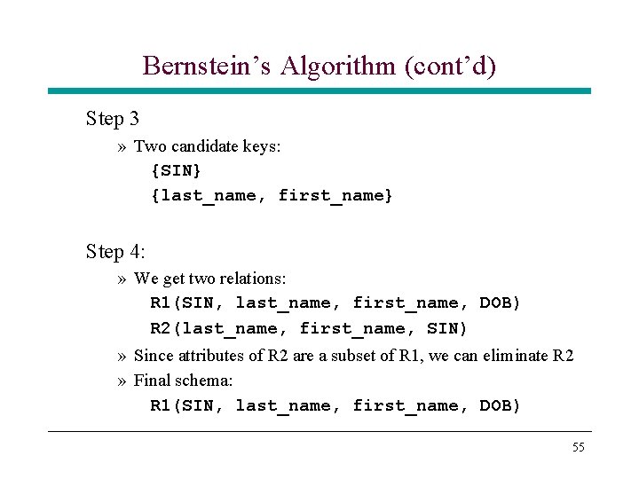
Bernstein’s Algorithm (cont’d) Step 3 » Two candidate keys: {SIN} {last_name, first_name} Step 4: » We get two relations: R 1(SIN, last_name, first_name, DOB) R 2(last_name, first_name, SIN) » Since attributes of R 2 are a subset of R 1, we can eliminate R 2 » Final schema: R 1(SIN, last_name, first_name, DOB) 55

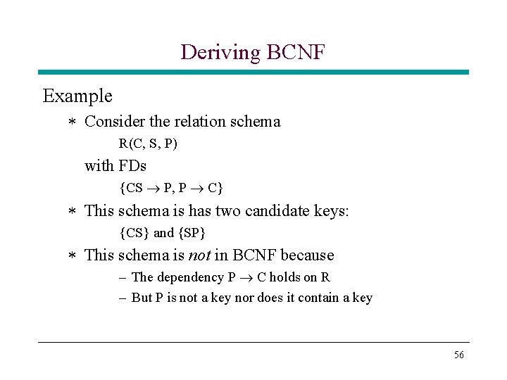
Deriving BCNF Example * Consider the relation schema R(C, S, P) with FDs {CS P, P C} * This schema is has two candidate keys: {CS} and {SP} * This schema is not in BCNF because – The dependency P C holds on R – But P is not a key nor does it contain a key 56

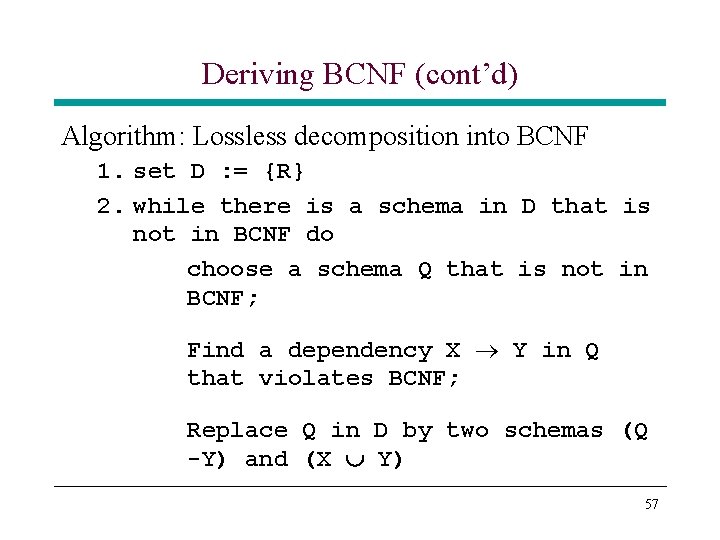
Deriving BCNF (cont’d) Algorithm: Lossless decomposition into BCNF 1. set D : = {R} 2. while there is a schema in D that is not in BCNF do choose a schema Q that is not in BCNF; Find a dependency X Y in Q that violates BCNF; Replace Q in D by two schemas (Q -Y) and (X Y) 57

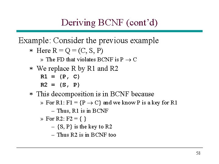
Deriving BCNF (cont’d) Example: Consider the previous example * Here R = Q = (C, S, P) » The FD that violates BCNF is P C * We replace R by R 1 and R 2 R 1 = (P, C) R 2 = (S, P) * This decomposition is in BCNF because » For R 1: F 1 = {P C} and we know P is a key for R 1 – Thus, R 1 is in BCNF » For R 2: F 2 = { } – {S, P} is the key to R 2 – Thus R 2 is in BCNF too 58

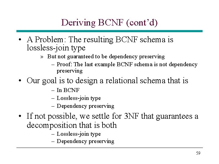
Deriving BCNF (cont’d) • A Problem: The resulting BCNF schema is lossless-join type » But not guaranteed to be dependency preserving – Proof: The last example BCNF schema is not dependency preserving • Our goal is to design a relational schema that is – In BCNF – Lossless-join type – Dependency preserving • If not possible, we settle for 3 NF that guarantees a decomposition that is both – Lossless-join type – Dependency preserving 59

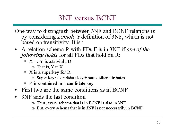
3 NF versus BCNF One way to distinguish between 3 NF and BCNF relations is by considering Zaniolo’s definition of 3 NF, which is not based on transitivity. It is : • A relation schema R with FDs F is in 3 NF if one of the following holds for all FDs that hold on R: * X Y is a trivial FD » That is, Y X * X is a superkey for R » Super key is candidate key + some other attributes * Y is contained in a candidate key • First two are the same conditions as in BCNF • 3 NF adds the last condition » Thus, every schema that is in BCNF is also in 3 NF » But, every schema that is in 3 NF is not necessarily in BCNF 60

4 NF Fourth normal form (4 NF) • Deals with a new type of dependency called multivalued dependency. Consider the following example: 61

4 NF (cont’d) Normalized table instance of CPT table is 62

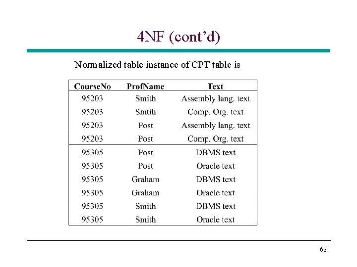
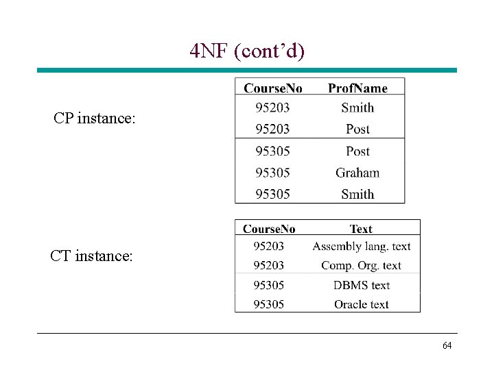
4 NF (cont’d) • Note that there is no functional dependencies for the data in CPT schema • CPT schema is in BCNF * All three attributes form the key to CPT relation • Redundancy in the data * Causes update anomalies * Inserting a new professor for 95305 requires two tuples • Intuitively, we know it is better if we split CPT into two relations by knowing that course was the key in the original relation R 1(C, P) R 2(C, T) 63

4 NF (cont’d) CP instance: CT instance: 64

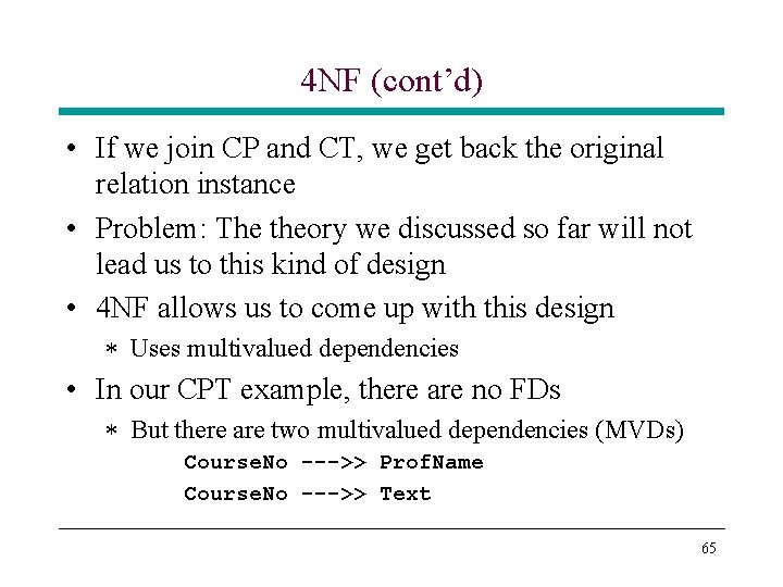
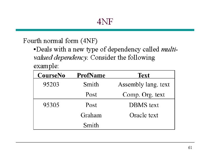
4 NF (cont’d) • If we join CP and CT, we get back the original relation instance • Problem: The theory we discussed so far will not lead us to this kind of design • 4 NF allows us to come up with this design * Uses multivalued dependencies • In our CPT example, there are no FDs * But there are two multivalued dependencies (MVDs) Course. No --->> Prof. Name Course. No --->> Text 65

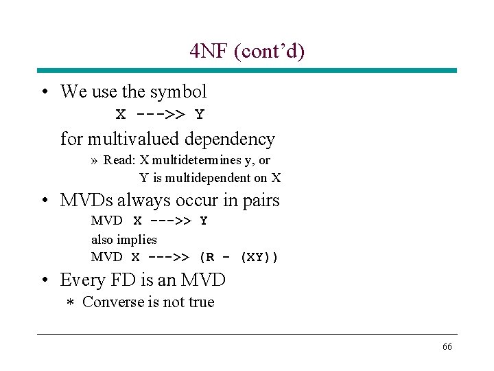
4 NF (cont’d) • We use the symbol X --->> Y for multivalued dependency » Read: X multidetermines y, or Y is multidependent on X • MVDs always occur in pairs MVD X --->> Y also implies MVD X --->> (R - (XY)) • Every FD is an MVD * Converse is not true 66

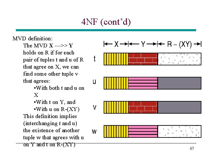
4 NF (cont’d) MVD definition: The MVD X --->> Y holds on R if for each pair of tuples t and u of R that agree on X, we can find some other tuple v that agrees: • With both t and u on X • With t on Y, and • With u on R-(XY) This definition implies (interchanging t and u) the existence of another tuple w that agrees with u on Y and t on R-(XY) 67

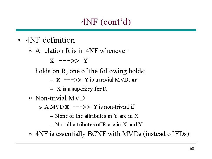
4 NF (cont’d) • 4 NF definition * A relation R is in 4 NF whenever X --->> Y holds on R, one of the following holds: – X --->> Y is a trivial MVD, or – X is a superkey for R * Non-trivial MVD » A MVD X --->> Y is non-trivial if – None of the attributes in Y are in X – Not all attributes of R are in X and Y * 4 NF is essentially BCNF with MVDs (instead of FDs) 68

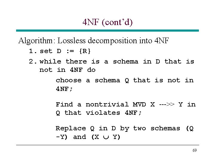
4 NF (cont’d) Algorithm: Lossless decomposition into 4 NF 1. set D : = {R} 2. while there is a schema in D that is not in 4 NF do choose a schema Q that is not in 4 NF; Find a nontrivial MVD X --->> Y in Q that violates 4 NF; Replace Q in D by two schemas (Q -Y) and (X Y) 69

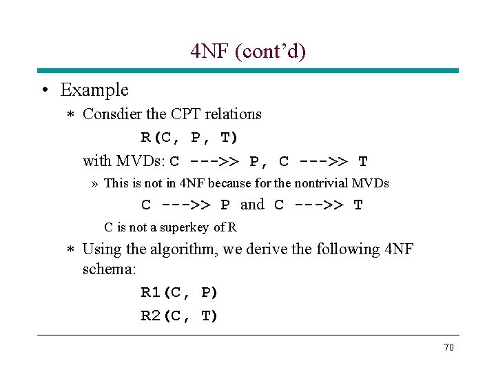
4 NF (cont’d) • Example * Consdier the CPT relations R(C, P, T) with MVDs: C --->> P, C --->> T » This is not in 4 NF because for the nontrivial MVDs C --->> P and C --->> T C is not a superkey of R * Using the algorithm, we derive the following 4 NF schema: R 1(C, P) R 2(C, T) 70

Additional Normal Forms • Additional normal forms also exist. For example 5 NF » 5 NF or PJNF (project-join normal form): deals with the relations that require to decompose into more than two relations to have lossless-join property » See Sections 13. 3 of the text (Date’s book) if you are interested • But BCNF/3 NF decomposition » Eliminates most of the anomalies » Allows for efficient checking of desired FDs 71